Two mathematical theorems connect probabilities with frequencies:
The Law of Large Numbers says that, in the long run, the probability of an event equals the frequency of its occurrence.
The Central Limit Theorem says that probabilities for the sum or average of a decent number of repeated events form a normal, bell-shaped curve.
Two-way Inference
The Law of Large Numbers is the basis for inferring frequencies from probabilities and probabilities from frequencies.
Inferring frequencies from probabilities:
The probability of rolling a seven in the game of craps is 1/6. You therefore expect that the more times you roll the dice the closer the frequency of sevens gets to 1/6.
Inferring probabilities from frequencies:
A million silver atoms are shot through a Stern-Gerlach magnet; 499,590 are deflected upwards, the rest downwards. The experiment is repeated six more times, with upwards deflection numbers of 500,087, 498782, 499368, 500768, 499808, and 499712. Thus, with 49.9% of atoms deflected upwards, the observed relative frequencies confirm the prediction of Quantum Mechanics that a silver atom passing through a Stern-Gerlach magnet is deflected upwards with probability 0.5.
Two Versions
There are two versions of the Law of Large numbers. The Strong Law logically implies the WeakLaw and is more transparent.
Strong Law of Large Numbers
The Strong Law of Large Numbers says:
Let X1, X2, …Xn be independent and identically distributed random variables, each having mean µ.
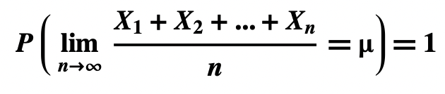
Then, with probability 1, the average of nXs approaches µ as n → ∞. That is:
Probability of 1?
When asked my name it would be for strange for me to say that the probability my name is Jim is 1. A probability of 1 means certainty. So I’ve said in effect that it’s certain my name is Jim. Which logically implies that that’s my name. So why not just say my name?
And why doesn’t the Strong Law merely assert that the limit of the average Xs equals the mean?
The answer is that the proposition that the limit equals the mean, by itself, is neither true or false.
Let X = the outcome of rolling a single die. X thus has the probability distribution:
P[X=1] = 1/6
P[X=2] = 1/6
P[X=3] = 1/6
P[X=4] = 1/6
P[X=5] = 1/6
P[X=6] = 1/6
Is X = 3 true or false?
The answer is: neither. The truth of X = 3 is indeterminate. X is defined by its probability distribution and therefore X = 3 has a determinate probability, 1/6. But neither the distribution nor anything else determines whether X = 3 is true or false.
The same goes for (X1 + X2) / 2 = 3.5
The same also goes for:
The limit of the average of nXs is a random variable and therefore the proposition that it equals μ, like X = 3 and (X1 + X2) / 2 = 3.5, has a probability but no truth-value. The Strong Law of Large Numbers is true (or false) only if the limit proposition is within a probability statement of the form P(…..) = n.
Strong Law for Small n
The Strong Law says that, with probability 1, the limit of the average of n instances of random variable X equals the mean of X, as n → ∞.
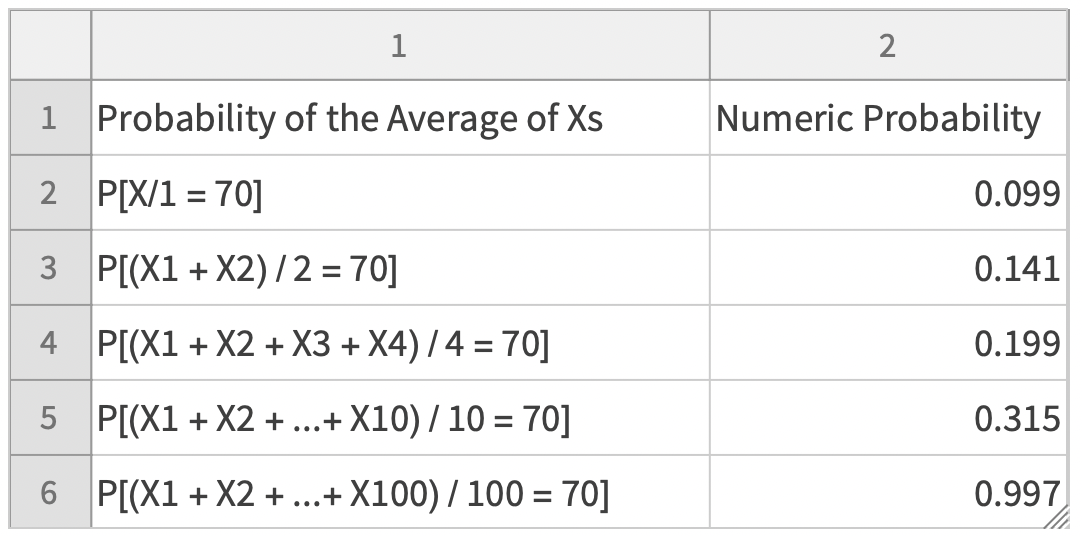
Let X = the outcome of measuring the height of a randomly selected male adult. We’ll assume that X is normally distributed with mean 70 and standard deviation 4.
Here are the probabilities that the average of n instances of X equals 70, for n = 1, 2, 4, 10, and 100.
It doesn’t take many instances of X for the probability to get close to 1.
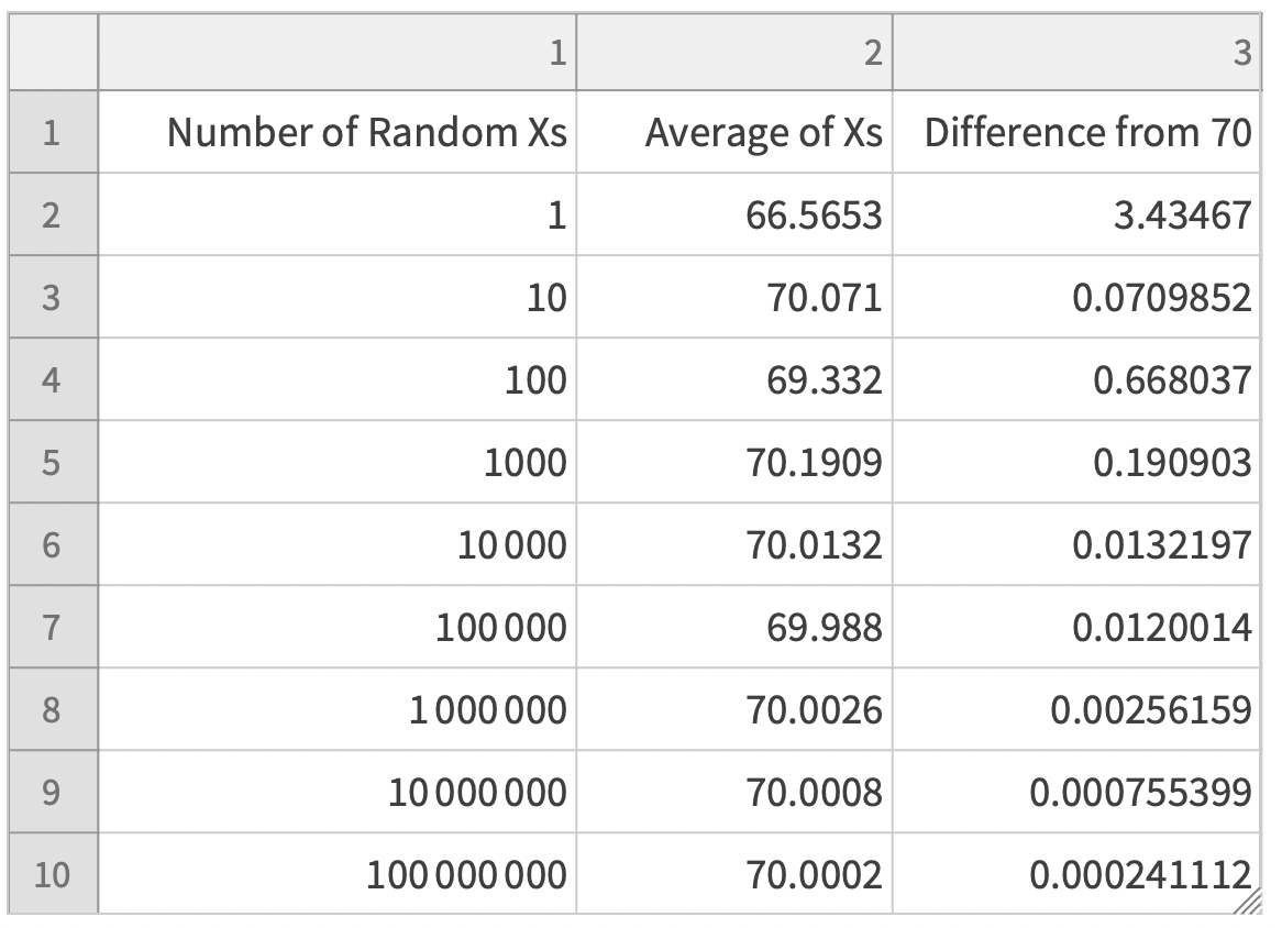
Simulation
With X equal to the outcome of measuring the height of a random male adult, we can simulate taking a random sample of n male adults and computing the average. The average, predictably, gets closer to 70 as n gets larger.
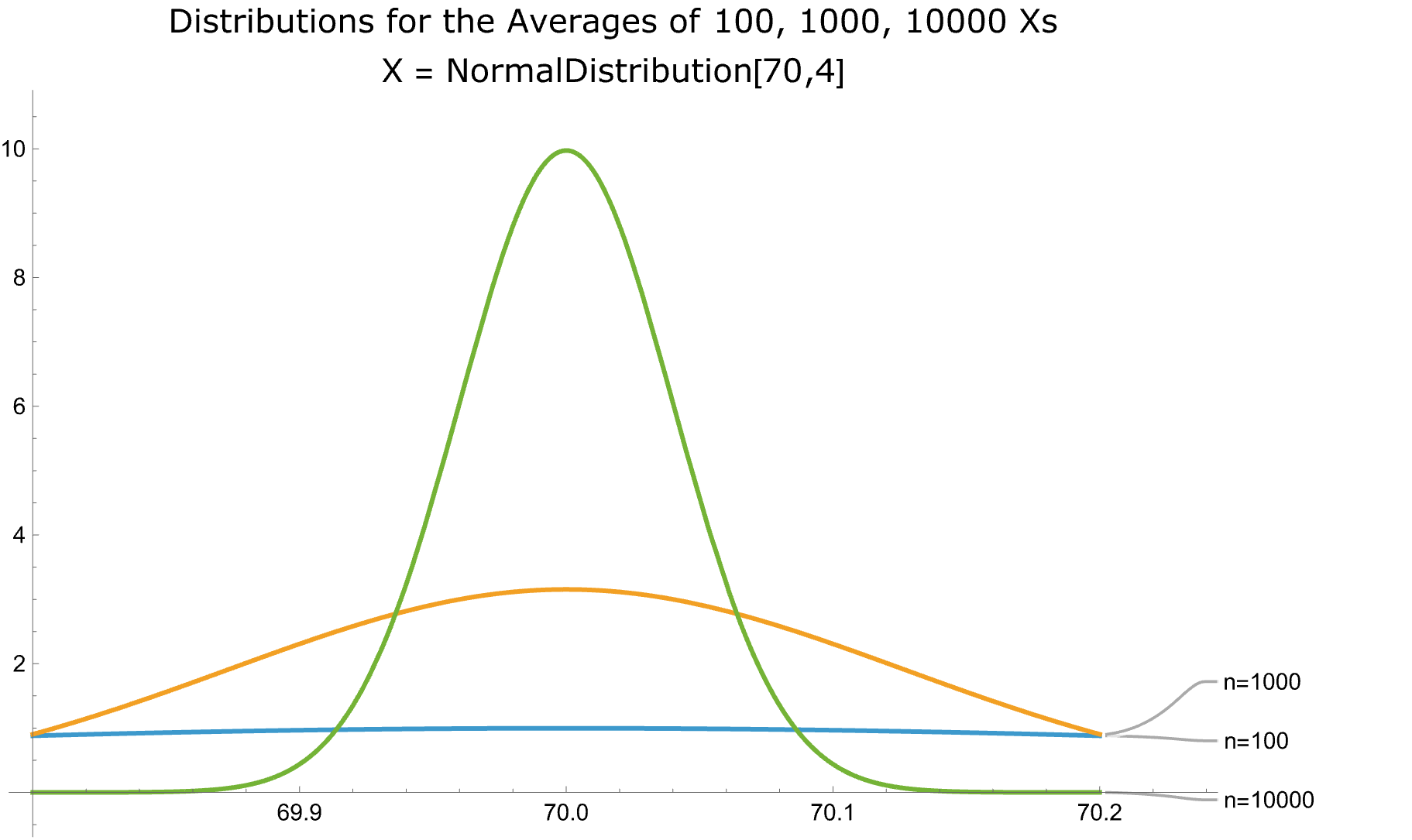
Plot of Many Xs
As n gets larger, the probability distribution of the average of nXs becomes more concentrated about the mean, the standard deviation shrinks, and the probability that the average = 70 gets closer to 1.
Weak Law of Large Numbers
The Weak Law of Large Numbers says:
Let X1, X2,…, Xnbe a sequence of independent and identically distributed random variables, each with mean μ.
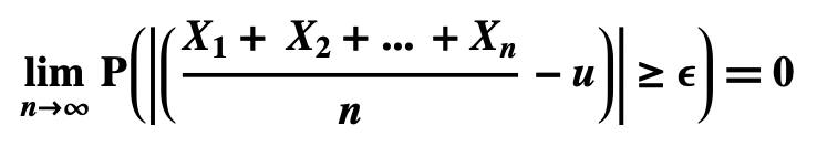
Then, for every ε > 0,
Format of the Weak Law
Format of the Weak Law, from the top down:
For every ε (….)
Limit of […] = 0 as n → ∞
P(Δn ≥ ε)
P = “the probability that”
Δn is a random variable for the absolute difference between the average of n Xs and the mean of X
Putting the pieces together:
For every ε ( Limit of [ P(Δn ≥ ε) ] = 0 as n → ∞ )
That is:
For every ε, the limit of [the probability that Δn ≥ ε] = 0 as n → ∞
Example
Let X be a normally distributed random variable with mean = 70 and standard deviation = 4.
Let ε = 1
Probabilities that |(X1 + X2 + …+ Xn)/n – 70| ≥ 1 for n = 2, 10, and 20:
P(|(X1 + X2)/2 – 70| ≥ 1)= 0.72
P(|(X1 + X2 + X3 + X10)/10 – 70| ≥ 1) = 0.43
P(|(X1 + X2 +…+ X20)/20 – 70| ≥ 1) = 0.26
And in the limit as n → ∞:
P(|(X1 + X2 +…+ Xn)/n – 70| ≥ 1)= 0
Let ε = 0.1.
Probabilities that |(X1 + X2 + …+ Xn)/n – 70| ≥ 0.1 for n = 2, 10, and 20:
P(|(X1 + X2)/2 – 70| ≥ 0.1) = 0.97
P(|(X1 + X2 + X3 + X10)/10 – 70| ≥ 0.1)= 0.94
P(|(X1 + X2 +…+ X20)/20 – 70| ≥ 0.1)= 0.91
And in the limit as n → ∞:
P(|(X1 + X2 +…+ Xn)/n – 70| ≥ 0.1)= 0
Thus in general:
Let Δn be the absolute difference between the average of n Xs and the mean of X.
For a fixed n, as ε gets smaller the probability that Δn ≥ ε gets larger.
For a fixed ε, as n gets larger, the probability that Δn ≥ ε gets smaller.
Difference Between Strong and Weak Laws
Here’s a thought experiment that perhaps sheds light on the difference between the weak and strong laws.
Let X = the outcome of rolling a single die. The mean of X is 3.5.
Pretend the limit is reached at n = 10.
What can we infer from the two laws?
Strong Law
The probability that average of 10 Xs = 3.5 equals 1.
Therefore, the average of 10 Xs = 3.5.
Weak Law
The probability that the difference between the average of 10 Xs and 3.5 ≥ ε equals 0.
So, there’s no chance that the difference ≥ ε.
So the difference = 0 ± ε.
So the average of 10 Xs = 3.5 ± ε
That is, for any ε > 0, the average of 10 Xs = 3.5 ± ε
Perhaps, then, we can say that the difference amounts to this:
The Strong Law says that, in the limit, the average of nXs equals the mean.
The Weak Law says that, in the limit, the average of nXseffectively equals the mean.