Random Variables and Probability Distributions

Contents

Specifying Numeric Probabilities

Individual Probability
- In rolling a pair of dice the probability of rolling a seven = ⅙
Probability Range
- In rolling a pair of dice the probability of rolling 5 through 9 = ⅔
- In rolling a pair of dice the probability of rolling at least 10 = ⅙
Probability Distribution
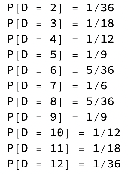
- In rolling a pair of dice the probabilities of rolling 2, 3, 4, 5, 6, 7, 8, 9, 10, 11, 12 are 1/36, 1/18, 1/12, 1/9, 5/36, 1/6, 5/36, 1/9, 1/12, 1/18, 1/36 respectively.

Probability Distributions

A probability distribution is an assignment of probabilities to a set of numbers.
- The Rolling Dice distribution assigns probabilities to the possible outcomes of a roll, the integers 2 through 12.

At the heart of a probability distribution are two functions:
- PDF, the probability density (or mass) function, returns the probability of the input value.
- CDF, the cumulative density (or mass) function returns the probability of values less than or equal to the input value.
For example, for Rolling Dice:
- Probability of Boxcars:
  - PDF(Rolling Dice, 12) = 1/36
- Probability of 7 or 11:
  - PDF[Rolling Dice, 7] + PDF[Rolling Dice, 11] = 2/9
- Probability of x ≥ 10:
  - 1 – CDF[Rolling Dice, 9] = ⅙
- Probability of x ≥ 7 & x ≤ 11:
  - CDF[Rolling Dice, 11] – CDF[Rolling Dice, 6] = 5/9

Probability distributions are discrete or continuous.
- A discrete distribution assigns probabilities only to a finite (or countable) set of numbers. For example, the Rolling Dice distribution assigns probabilities to the integers 2 through 12 but not to the real numbers between.
- A continuous distribution assigns probabilities to real numbers. The normal distribution, for instance, assigns probabilities to all real numbers from negative infinity to positive infinity.

Every probability distribution is characterized by a set of numeric properties, the most important being mean, variance, standard deviation, and quintile. For Rolling Dice, for example:
- Mean = 7
- Variance = 35/6
- Standard deviation = √(35/6)
- Quartiles = {5, 7, 9)
- Quantile[0.1] = 4
- Quantile[0.9] = 10

A probability distribution is not a frequency distribution. The latter is a calculation on the data. A probability distribution, on the other hand, is a self-contained abstract entity.

The terms mean, variance, standard deviation, and quantile have dual senses. They have one meaning when applied to datasets. They have a different but analogous meaning when applied to probability distributions and random variables. For example, the mean of ten rolls of a pair of dice is the sum of the ten rolls divided by ten. But the mean of Rolling Dice is the probability-weighted average of the possible outcomes. The former is a calculation on a dataset, varying from one dataset to another. The latter is an a priori calculation on an abstract entity and is fixed at seven.

Random Variables

Random variables provide the symbolism for stating and proving theorems about probability distributions.
A random variable, typically a capital letter, is defined by a probability distribution, which assigns probabilities to its values. It can be thought of as the outcome of a probabilistic process.
For example, let random variable D = the outcome of rolling a pair of dice. D’s values are the integers 2 through 12 with the probabilities:
A tilde is used to specify a random variable’s probability distribution. Thus:
- D ~ Rolling Dice.
A random variable is discrete or continuous, depending on its probability distribution. D is discrete.
And a random variable has the numeric properties of its probability distribution. Thus the mean of D is 7, that of Rolling Dice.
Statements with random variables have determinate probabilities but no truth-values. That’s because a random variable’s probability distribution determines probabilities, not truth and falsehood. Thus, the probability that D ≤ 12 is 1. But it’s a mistake think that D ≤ 12 is true.

Three Common Distributions

Scientists have developed hundreds of parametric probability distributions, i.e. those that take parameters. Distributions such as:
- Discrete
  - Bernoulli (probability of success)
  - Binomial (number of trials, probability of success)
  - Poisson (mean)
  - Discrete Uniform (minimum integer, maximum integer)
  - Geometric (probability of success)
  - Hypergeometric(number of draws, number of successes, population size)
- Continuous
  - Normal (mean, standard deviation)
  - Student T (degrees of freedom)
  - ChiSquare (degrees of freedom)
  - Continuous Uniform (minimum real number, maximum real number)
  - Exponential (parameter)
  - Βeta (shape, shape)
  - Gamma (shape, scale)
See wikipedia.org/wiki/List_of_probability_distributions for a long list.
I briefly discuss three: the binomial, Poisson, and normal distributions.

Binomial Distribution

The binomial distribution gives the probabilities of the possible outcomes of a series of trials, where the outcome of each trial is:
1. binary, e.g. success or failure, heads or tails, 1 or 0.
2. determined by the same probability.
The distribution takes two parameters:
- n = the number of trials.
- p = the probability of success on a given trial.
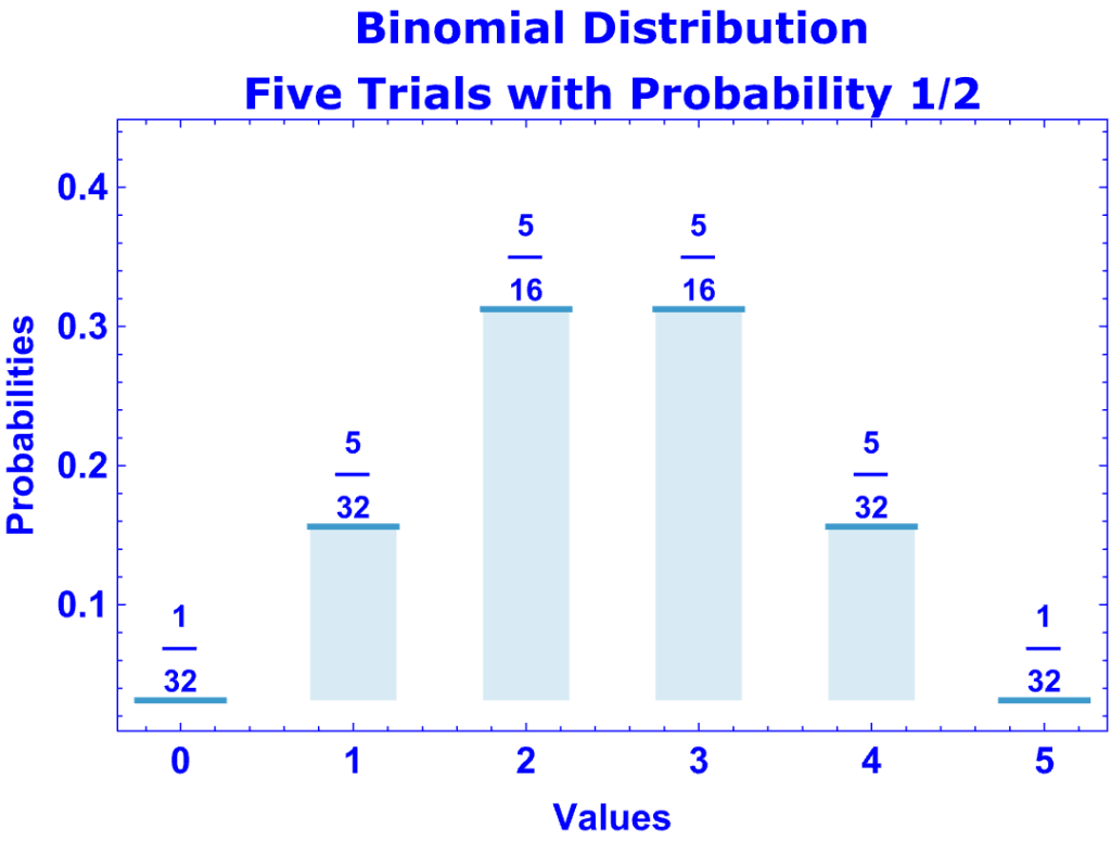
The graph, for example, represents the binomial distribution for the number of heads in five tosses of an unbiased coin.

Poisson Distribution

The Poisson distribution is a discrete probability distribution that’s been found to approximate very unlikely events occurring randomly within a given time or space.
The distribution takes one parameter: the mean of the distribution. Its variance is the same as the mean.
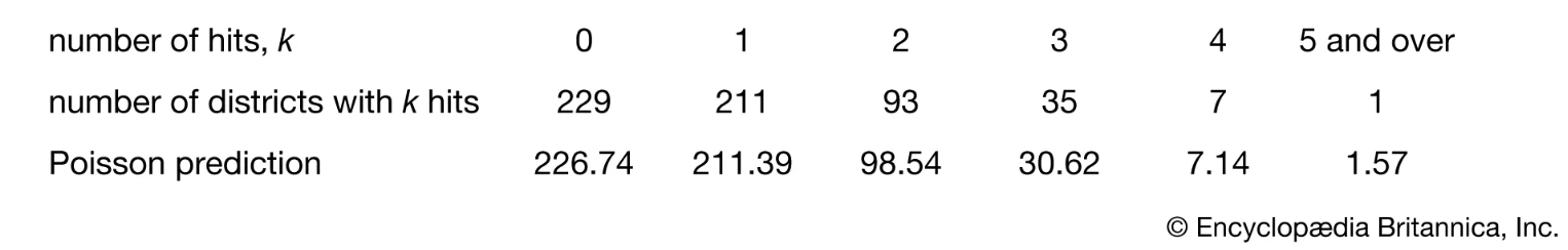
The Britannica relates the story of R. D. Clark who, during WWII, was asked to determine whether the V-1 and V-2 rockets hitting London were targeted to hit certain locations or were hitting locations randomly. He divided London into small equally-sized plots and recorded the number hits in each. The Poisson distribution approximated the number of plots with 0, 1, 2, 3, 4, and 5 hits.
Clark concluded that the rockets were hitting London randomly.
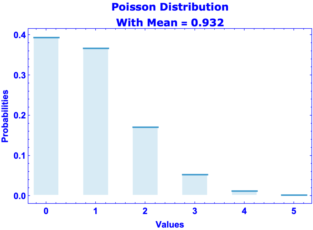
Here’s a graph of my reconstruction of Clark’s Poisson distribution.

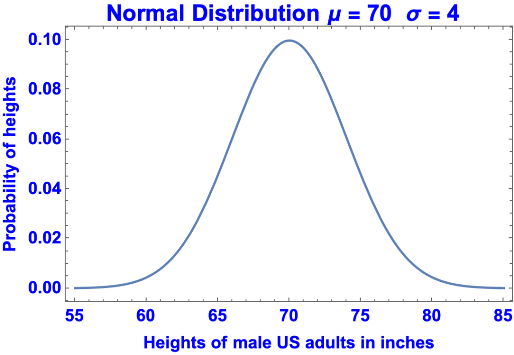
Normal Distribution

The normal distribution is a continuous, bell-shaped, symmetric distribution that approximates natural quantities such as blood pressure, income, and measurement errors.
The distribution takes two parameters:
- μ = the mean of the distribution
- σ = the standard deviation of the distribution
The graph depicts the normal distribution that approximates adult male heights in inches.

Mean of a Random Variable and Expectation

The mean of a random variable (or probability distribution) is the sum (or integral) of its probability-weighted values.
For a discrete random variable X,
- the mean of X = the sum of (X · P(X)) for all values of X.
For a continuous random variable X,
- the mean of X = the integral of (X · P(X)) for all values of X.
For example, the means of Rolling Dice, the Binomial Distribution[5, 0.5], and the Normal Distribution[70,4] are:

The mean of a random variable is also its expectation (or expected value). Expectation applies not just to random variables but to functions of random variables as well. Thus, not only is E(D) = 7, but E(2D) = 14, and E(D²) = 329 / 6.

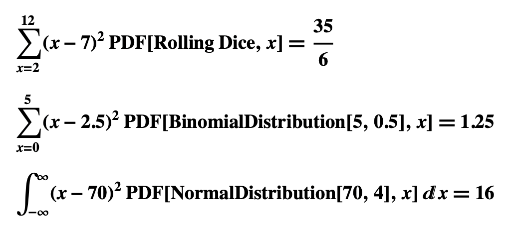
Variance and Standard Deviation of a Random Variable

The variance of a random variable (or probability distribution) is the sum (or integral) of the probability-weighted “square-distance” of its values from the mean.
For a discrete random variable X,
- the variance of X = the sum of ((X – μ)²· P(X)) for all values of X, where μ is the mean of X.
For a continuous random variable X
- the variance of X = the integral of ((X – μ)²· P(X)) for all values of X, where μ is the mean of X.
Thus, for example, the variances of Rolling Dice, the Binomial Distribution[5, 0.5], and the Normal Distribution[70, 4] are:
In the language of random variables, Var(X) = E[(X – μ)²].

It’s easily shown, moreover, that Var(X) = E(X²) – (E(X))². For example:

Finally, the standard deviation of a random variable (or probability distribution) is the square root of its variance.
Thus, the standard deviations of Rolling Dice, the Binomial Distribution[5, 0.5], and the Normal Distribution[70, 4] are: √(35/6), 1.118, and 4 respectively.