Contents
- The Limit Theorems
- The Central Limit Theorem in a Nutshell
- Informal Version
- Mathy Version
- Applications
- CLT and the Justification of Statistical Estimation
- Computer Simulation for the Exponential Distribution
The Limit Theorems
- Two mathematical theorems connect probabilities with frequencies:
- The Law of Large Numbers says that, in the long run, the probability of an event equals the frequency of its occurrence.
- The Central Limit Theorem says that probabilities for the sum or average of a decent number of repeated events form a normal, bell-shaped curve.
- Both are stated in terms of a sequence of random variables that are independent and have the same probability distribution. Both assert that something is true in the limit as the length of the sequence approaches infinity.
The Central Limit Theorem in a Nutshell
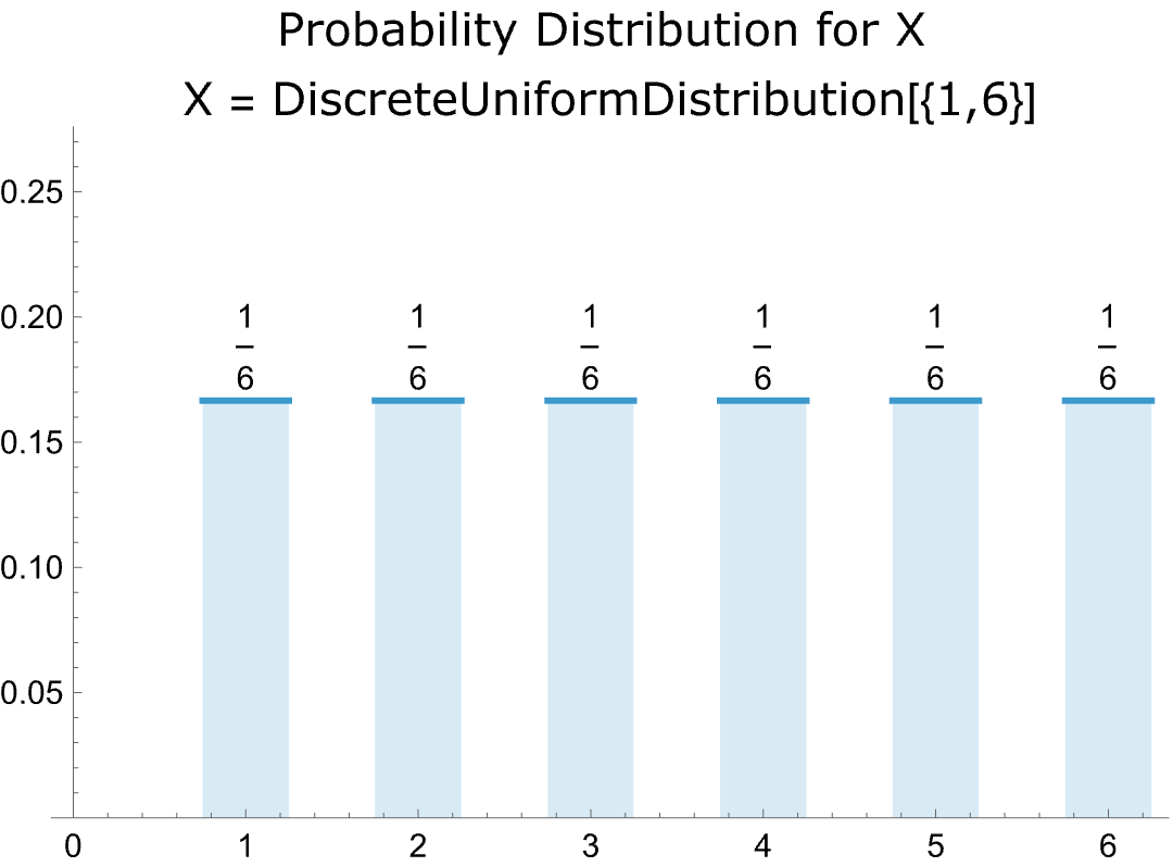
- Roll a single die and the probability of each outcome is 1/6.
- The plot of the probabilities is thus flat:
-
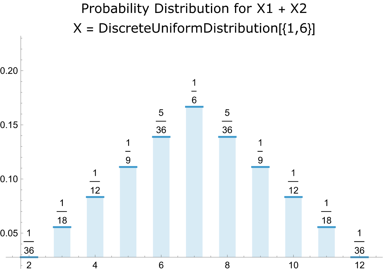
- Rolling two dice is a different matter. The plot of the probabilities is a bell-shaped curve.
-
- So how does a bell-shaped curve of probabilities emerge from two sets of flat probabilities?
- The answer: there are more combinations of outcomes around the middle of the distribution.
- There’s only one way of rolling a two with a pair of dice. So the probability is 1/6 x 1/6 = 1/36.
- There are three ways of rolling a four: L1 + R3, L2 + R2, and L3 + R1, where L = left die and R = right die. In each case the probability is 1/6 x 1/6 = 1/36. So the probability of rolling a four = 3 x 1/36 = 1/12.
- And there are six ways of rolling a seven: L1 + R6, L2 + R5, L3 + R4, L4 + R3 + L5 + R2, L6 + R1. The the probability in this case = 6 x 1/36 = 6/36.
- The Central Limit Theorem says that the same mechanism is at work whenever independent instances of a probability distribution are added; that is, there are more combinations of outcomes toward the center of the distribution and therefore higher probabilities. Indeed, per the CLT, if enough instances are added, the distribution of the sum of is approximately normal.
- Here, for example, is the probability distribution for rolling four dice with the appropriate normal distribution superimposed.
-
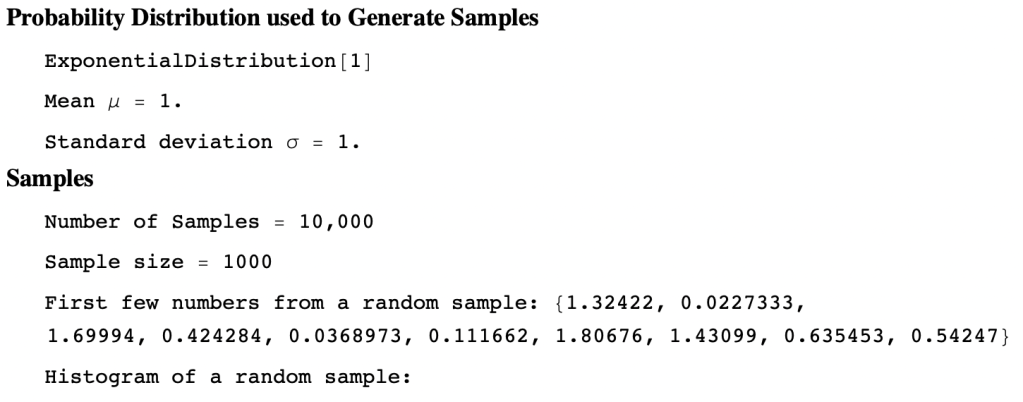
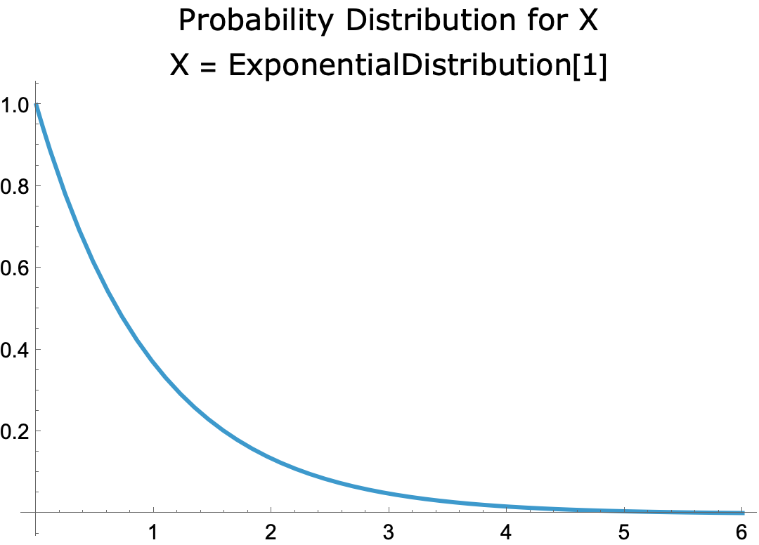
- Here’s the graph of a very different probability distribution, the exponential distribution with parameter = 1.
-
- The probability that X = 0 equals 1 and the probability for X > 0 trails off to 0.
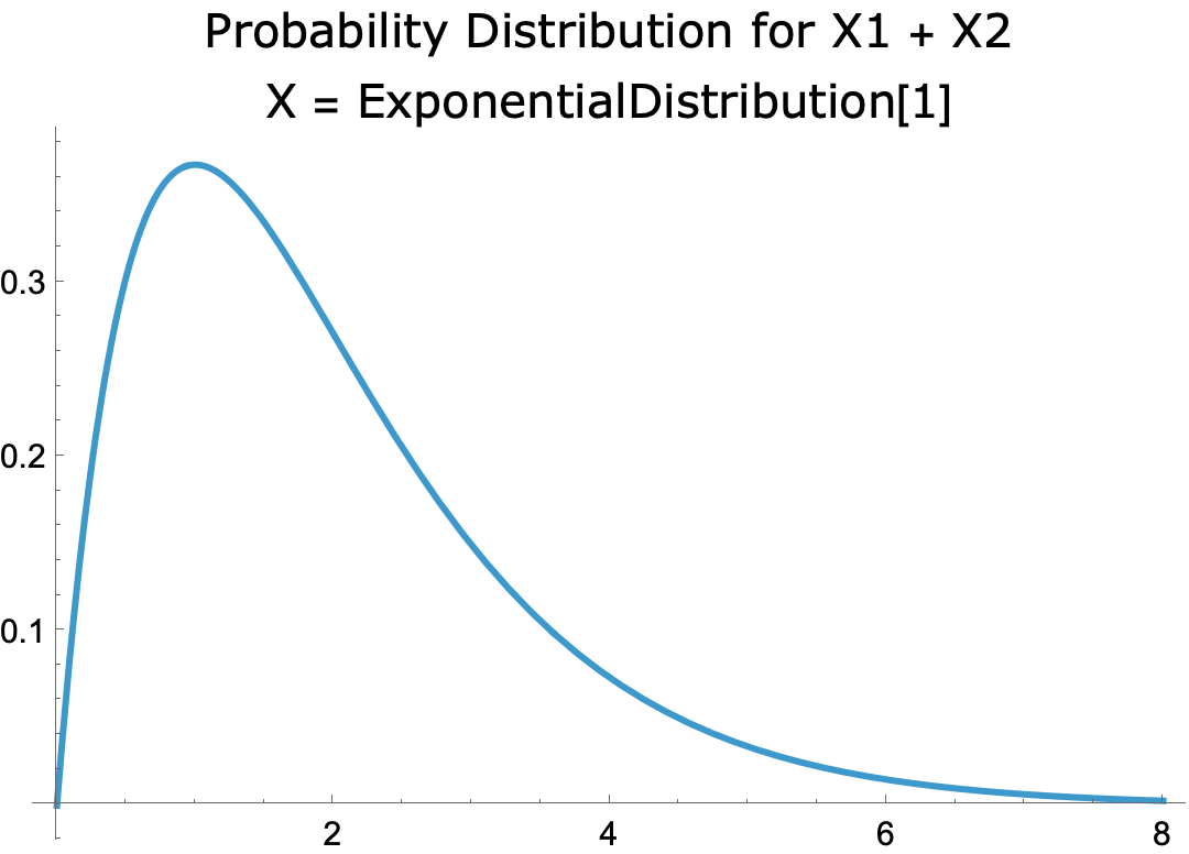
- The distribution of the sum of two exponential distributions has a skewed bell-shaped curve.
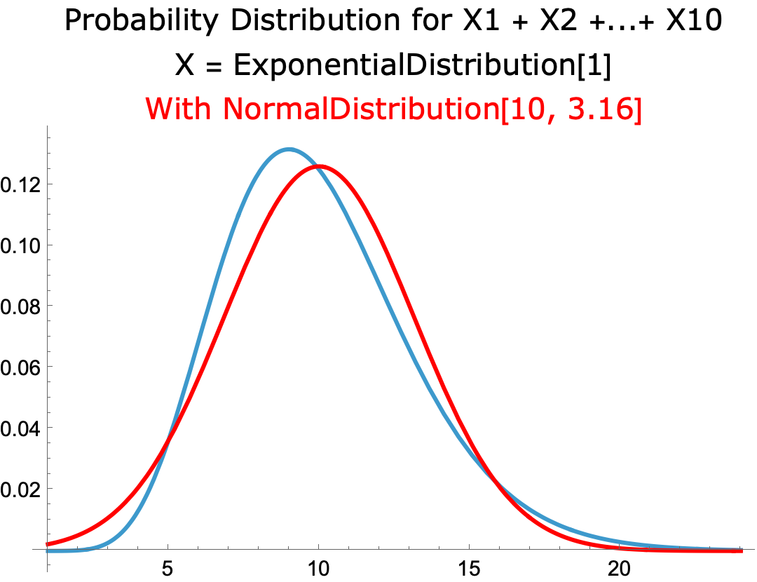
- For the sum of ten exponential distributions, the probability distribution is close to the normal distribution with mean = 10 and standard deviation = 3.16
-
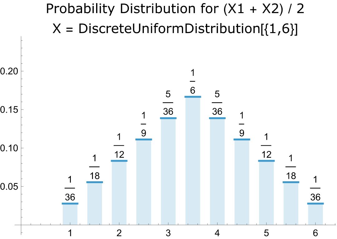
- The CLT applies not only to the sum of instances of a probability distribution but to their average as well. Here, for example, is the graph of the average of rolling two dice:
-
- The graph resembles that for rolling a single die but includes, in addition, outcomes halfway between the integers, since, for example, the average of rolling a one and a two is 1.5.

Informal Version
- The probability distribution of the sum (or mean) of a decent number n of independent random variables, each with mean μ and standard deviation σ, is approximately normal, regardless of the distribution. Moreover:
- For the sum of the random variables, the normal distribution has mean = nμ and standard deviation σ√n.
- For the mean of the random variables, the normal distribution has mean = μ and standard deviation σ/√n.
Mathy Version
- Let X1, X2,…,Xn be independent and identically distributed random variables, each with mean = μ and standard deviation σ. Then, for any real number 𝒂,
- where
- where either
- or
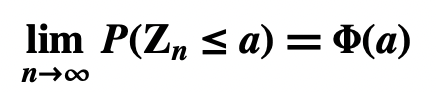

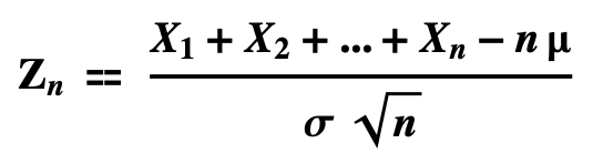
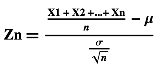
Illustration of the Mathy (Average) Version of CLT using Mathematica
- Suppose a box consists of a vast number of tickets, 80 percent of which are marked with the numeral “1” and the rest with the numeral “0”.
- Let X be the number of a ticket randomly selected from the box.
- The probability that X = 1 is 0.8 and the probability that X = 0 is 0.2. That is
- P(X=1) = 0.8
- P(X=0) = 0.2
- The probability distribution of X is the Bernoulli Distribution:
- X ~ Bernoulli Distribution[0.8].
- The mean and standard deviation of X are 0.8 and 0.4:
- Mean[BernoulliDistribution[0.8]] = 0.8
- StandardDeviation[BernoulliDistribution[0.8]] = 0.4
- We randomly draw 5 tickets from the box (with replacement).
- Let X5 be the result of averaging five random draws from the box. In Mathematica we can define the probability distribution for X5 as follows:
- X5 =TransformedDistribution[(u1+u2 + u3+u4 + u5) / 5,
- {u1 [Distributed]BernoulliDistribution[0.8],
- u2 [Distributed]BernoulliDistribution[0.8],
- u3 [Distributed]BernoulliDistribution[0.8],
- u4 [Distributed]BernoulliDistribution[0.8],
- u5 [Distributed]BernoulliDistribution[0.8]}];
- X5 =TransformedDistribution[(u1+u2 + u3+u4 + u5) / 5,
- The mean and standard deviation of X5 are:
- N[Mean[X5]] = 0.8
- N[StandardDeviation[X5]] = 0.178885
- Since X has values 1 and 0, the values of X5 run from 0 to 1. The mean and standard deviation of X5 are thus the mean and standard deviation of numbers such as 0, 0.2, 0.4, 0.6, 0.8, and 1.
- The first part of CLT says that the standard deviation of X5 equals the standard deviation of the Bernoulli distribution (0.4) divided by the square root of the number of tickets (5):
- 0.4 /√5 = 0.178885
- Next we “standardize” X5 by subtracting from the average of the five draws the mean of the Bernoulli Distribution (0.8) and dividing the result by the standard deviation of the Bernoulli Distribution divided by the square root of the number of tickets (0.4 /√5):
- X5z =TransformedDistribution[((u1+u2 + u3+u4 + u5)/5 – 0.8)/(0.4/√5),
- {u1 [Distributed]BernoulliDistribution[0.8],
- u2 Distributed]BernoulliDistribution[0.8],
- u3 [Distributed]BernoulliDistribution[0.8],
- u4 [Distributed]BernoulliDistribution[0.8],
- u5 [Distributed]BernoulliDistribution[0.8]}];
- X5z =TransformedDistribution[((u1+u2 + u3+u4 + u5)/5 – 0.8)/(0.4/√5),
- The mean and standard deviation of X5z are 0 and 1:
- N[Mean[X5z]] = 0
- N[StandardDeviation[X5z]] = 1
- The second part of CLT says that, in the limit, as the number of tickets approaches infinity, the standardized distribution becomes the standard normal distribution. Here’s what the cumulative probabilities for X5z and the standard normal distribution look like.
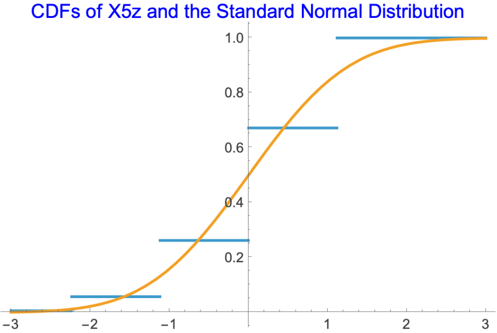
- As the number of tickets increases, the number of the blue horiztonal lines of X5z increases and their length decreases, gradually merging into the orange, curved line of the normal distribution.
Applications
Basis for Inferring a Population Parameter from a Sample Statistic
- The foremost application of the Central Limit Theorem is the essential role it plays in justifying the inference from a sample statistic to a population parameter.
- Hypothetico-deductive Confirmation is the view that a scientific theory is supported or disproved by its predictions. Einstein’s General Relativity, for example, is supported by its prediction of gravity waves. Newton’s theory of gravitation, by contrast, is refuted by its prediction that gravitational attraction is instantaneous. Per HD Confirmation, a poll supports an inferred hypothesis because the hypothesis predicts the results of the poll. The Central Limit Theorem is essential in deriving the prediction from the hypothesis.
- See CLT and the Justification of Statistical Estimation.
Basis for Confidence Levels and Intervals
- The Central Limit Theorem provides the theoretical basis for confidence levels and intervals.
- Estimating a Proportion, an Example
- The poll
- 600 of 1,000 people in a random poll identify as religious.
- The sample statistic is thus the proportion 0.6.
- The results of the poll support the hypothesis that 60 percent of the population are religious.
- Call this hypothesis H.
- The Individual Probability Distribution
- Let X = the response of a randomly selected person asked whether they are religious.
- Given hypothesis H, X is defined by the Bernoulli [0.6] distribution:
- P[X=0]=0.4]
- P[X=1]=0.6]
- Given hypothesis H, X is defined by the Bernoulli [0.6] distribution:
- The mean of X is μ = 0.6.
- The standard deviation of X is σ = 0.49.
- Let X = the response of a randomly selected person asked whether they are religious.
- The Sampling Distribution
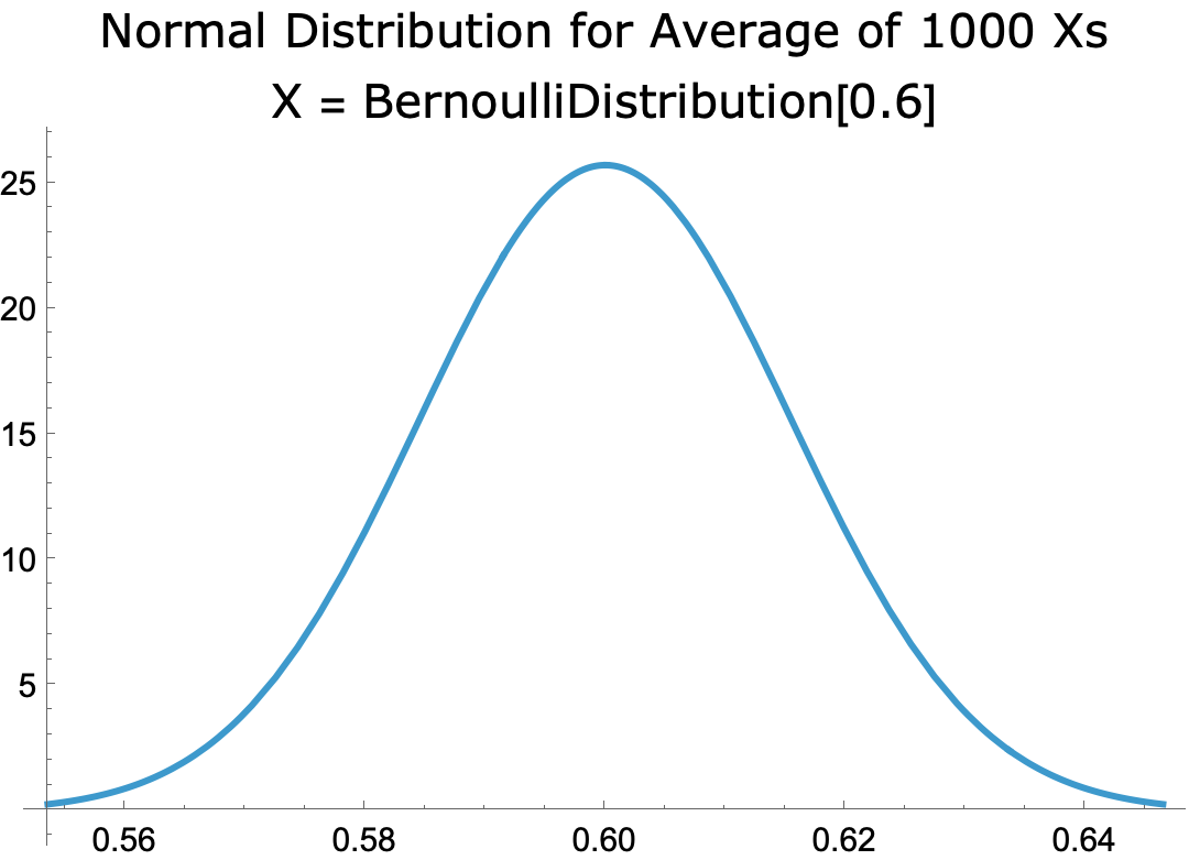
- The sampling distribution for the Bernoulli [0.6] Distribution, with n = 1000, is the probability distribution for the average of 1,000 independent instances of the distribution, which, per the CLT, is approximated by the normal distribution with mean μ = 0.6 and standard deviation σ /√n = 0.0155
- The distribution looks like this:
-
- The Standard Error, Margin of Error, and Confidence Intervals
- The standard error, SE, is the standard deviation of the sampling distribution, σ /√n = 0.0155
- Margins of error are defined by reference to the SE:
- 90% margin of error = 1.645 SE = 0.0255
- 95% margin of error = 1.96 SE = 0.03
- 99% margin of error = 2.575 SE = 0.04
- Confidence intervals and levels are defined by reference to the margins of error:
- The confidence interval at the 90 percent level = u ± the 90% margin of error = 0.6 ± 0.0255
- The confidence interval at the 95 percent level = u ± the 95% margin of error = 0.6 ± 0.03
- The confidence interval at the 99 percent level = u ± the 99% margin of error = 0.6 ± 0.04
- Thus, the confidence interval at the 95 percent level for the Bernoulli [0.6] distribution with n = 1000 is 60 percent ± 3 percentage points.
- Which means:
- There is a 95 percent probability that, in a random sample of 1000 people, between 57 and 63 identify as religious.
- The poll
- Estimating a Mean, an Example
- The Poll
- The heights of a random sample of 1,000 adult males are measured.
- The average height is found to be 70 inches.
- So the sample statistic is the mean 70.
- The results of the poll support the hypothesis that the average height of adult males in the population is 70 inches.
- Call this hypothesis H.
- The Individual Probability Distribution
- Let X = the outcome of a measuring the height of a randomly selected adult male.
- Given hypothesis H, X has a normal distribution with μ = 70 and σ = 4.
- The Sampling Distribution
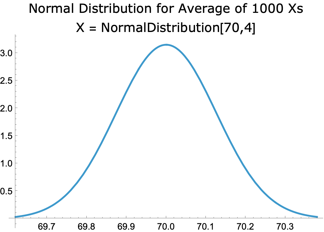
- The sampling distribution for the normal distribution [70,4], with n = 1000, is the probability distribution for the average of 1,000 independent instances of the distribution, which, per the CLT, is approximated by normal distribution with mean μ = 70 and standard deviation σ /√n = 0.126
- The distribution looks like this:
-
- The Standard Error, Margin of Error, and Confidence Intervals
- The standard error, SE, is the standard deviation of the sampling distribution, σ /√n = 0.126
- Margins of error are defined by reference to the SE:
- 90% margin of error = 1.645 SE = 0.21
- 95% margin of error = 1.96 SE = 0.25
- 99% margin of error = 2.575 SE = 0.33
- Confidence intervals and levels are defined by reference to the margins of error.
- The confidence interval at the 90 percent level = u ± the 90% margin of error = 70 ± 0.21
- The confidence interval at the 95 percent level = u ± the 95% margin of error = 70 ± 0.25
- The confidence interval at the 99 percent level = u ± the 99% margin of error = 70 ± 0.33
- Thus, the confidence interval at the 95 percent level for the normal distribution [70,4] with n = 1000 is 70 inches ± 0.25.
- Which means:
- There is a 95 percent probability that the average height of a random sample of 1,000 male adults is between 69.75 and 70.25 inches.
- The Poll
- Confidence intervals are not Bayesian credible intervals.
- The difference is that confidence intervals are about samples and credible intervals are about the population.
- Suppose that the average of height of a random sample of 1,000 adult males is 70 inches. Then:
- The confidence interval at the 95 percent level = 70 ± 0.25 means that there is a 95 percent probability that the average height of the people in a random sample of 1,000 adult males is 70 inches ± 0.25.
- The credible interval at the 95 percent level = 70 ± 0.25 means that there is a 95 percent probability that the average height of adult males in the population is 70 inches ± 0.25.
Computing Distributions for Sums and Averages of Many Independent Random Variables
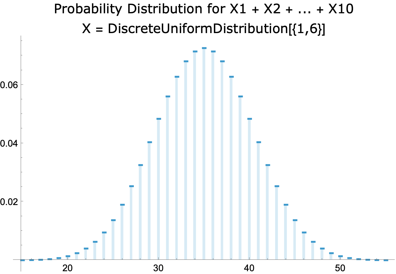
- A computer can easily compute probability distributions for the sum and average of 10 independent instances of a random variable. For example,
- Discrete uniform distribution from 1 to 6:
-
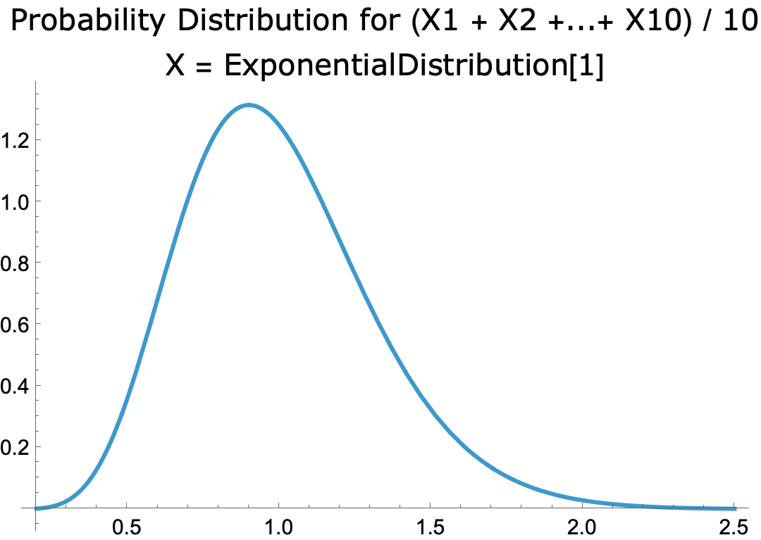
- Exponential distribution with parameter 1
-
- But when 1,000 iterations are involved processing time can tank, depending on the distribution.
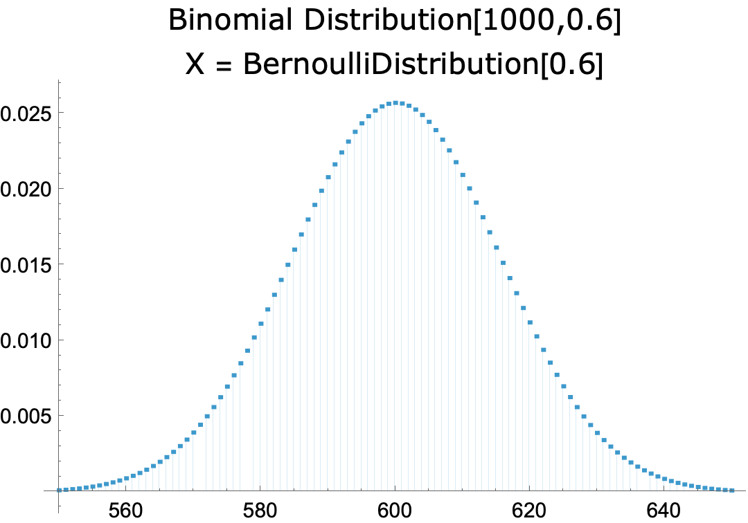
- Thus the distribution for the sum of 1,000 Bernoulli distributions is quickly calculated using the binomial distribution.
-
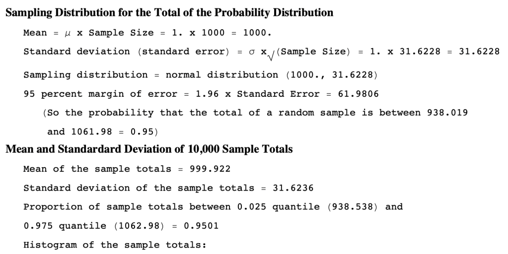
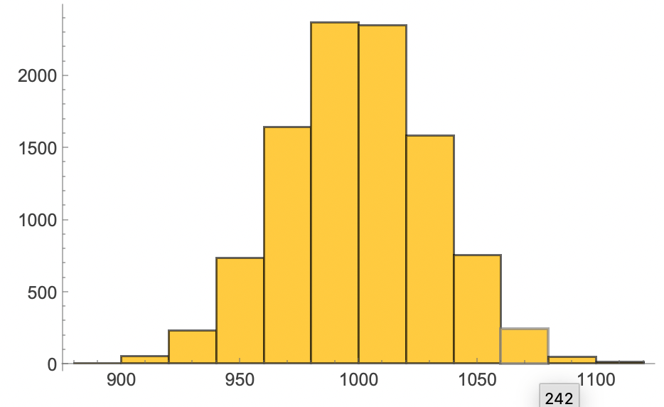
- But calculating the sum of 1,000 instances of the distribution for rolling a die is a different matter.
- For the sum of n instances, outcomes range from n to 6n. Thus outcomes go from 2 to 12 for rolling a pair of dice. For rolling 1,000 dice, outcomes run from 1,000 to 6,000. That’s a lot of computing.
- Thanks to the Central Limit Theorem, the distribution for rolling 1,000 dice is approximated by one that’s quickly computed: the normal distribution with mean = 1000 x 3.5 and standard deviation = 1.7 x √(1000)
-
- Likewise for the sum and average of a large number of iterations of any probability distribution.

CLT and the Justification of Statistical Estimation
- In Statistical Estimation a population parameter is inferred from a sample statistic.
- Inferring the mean of a measurable property
- The average of a certain measurable property (e.g. height) among members of a random sample = m.
- Therefore, the average of the property among members of the population = m.
- Inferring the proportion having a certain property
- The proportion of members of a random sample having a certain property (e.g. identifying as religious) = p.
- Therefore, the proportion of members of the population having the property = p.
- Inferring the mean of a measurable property
- The obvious (philosophic) question is: what justifies the inference from a poll of, say, a thousand people to a population of perhaps millions.
- Hypothetico-deductive Confirmation is the view that a scientific theory is supported or disproved by predictions derived from its postulates (typically supplemented by auxiliary assumptions). Einstein’s General Relativity, for example, is supported by its prediction of gravity waves. The Big Bang Theory is supported by its prediction of the CMB radiation. And, per HD Confirmation, a random sample supports an inferred hypothesis about the population because the hypothesis predicts the results of the sample.
- Example:
- Suppose a random poll of 1,000 people is conducted, 600 of whom identify as religious.
- It’s estimated based on the poll that 60 percent of the population is religious. Let’s call this hypothesis H.
- Per HD Confirmation, the results of the poll support H because H predicts the results.
- The prediction is derived from H using the Central Limit Theorem.
- Let X be the outcome of a randomly selected person asked whether they’re religious. Given hypothesis H, X has the following probability distribution (where 1 = identifies as religious):
- P[X=0] = 0.4
- P[X=1] = 0.6
- Let μ and σ be the mean and standard deviation of X.
- Per the CLT, the probability distribution of the sum of 1,000 independent Xs is approximated by the normal probability distribution with mean = 1000μ and standard deviation = σ√1000.
- The probability that x is 600±30 under such a distribution is 95%.
- Therefore, there is a 95% probability that, in a random poll of 1,000 people, between 570 and 630 identify as religious.
- Let X be the outcome of a randomly selected person asked whether they’re religious. Given hypothesis H, X has the following probability distribution (where 1 = identifies as religious):
- Any poll in this range supports H. Any poll outside the range is evidence against H.
- Our hypothetical poll is in this range.
- Therefore, the hypothetical poll supports H.
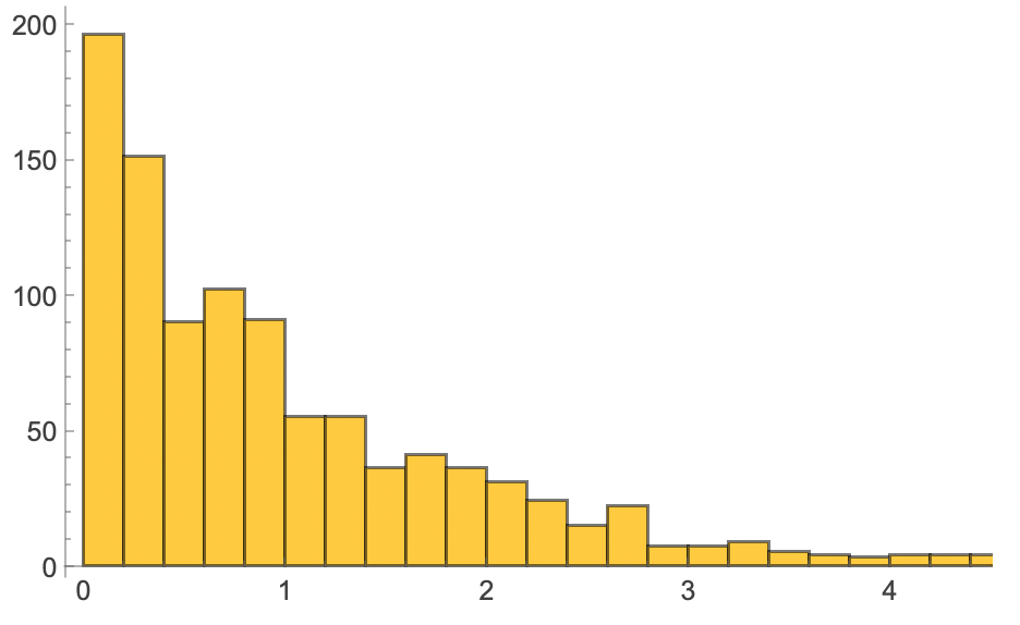
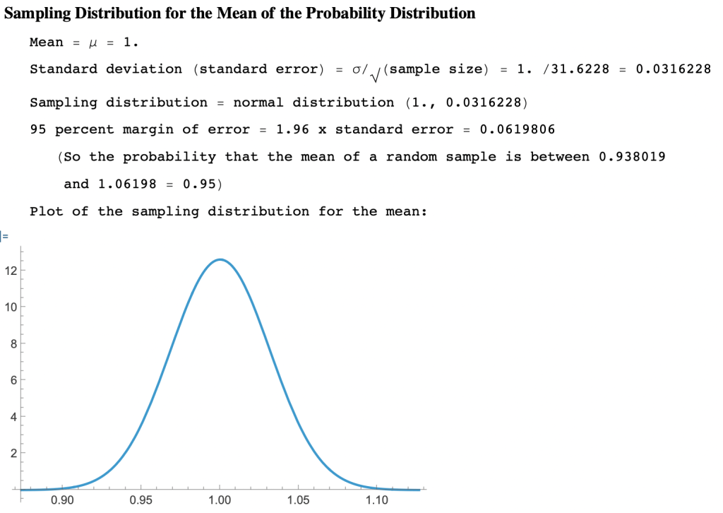
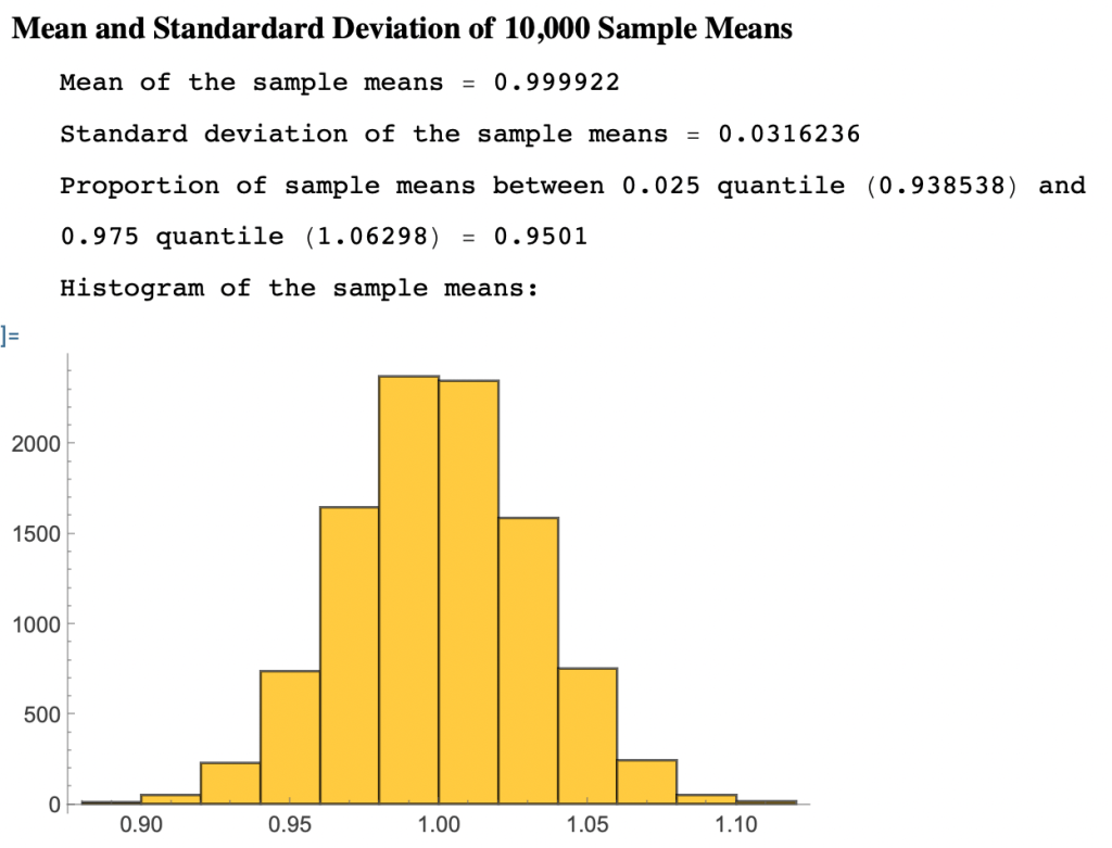
Computer Simulation for the Exponential Distribution