Contents
- Statistical Estimation
- Basic Form of Argument
- Justification
- Calculations of Confidence Levels and Intervals
- Monte Carlo Simulation of 95% Confidence Level
- Bayesian Estimation
- Comparison of Standard Error with Standard Deviation of Simulated Samples
Statistical Estimation
- Statistical Estimation is the statistical procedure for inferring the value of a population parameter from a random sample, e.g. a president’s approval rating based on a poll.
Basic Form of Argument
- A statistic S for a random sample from a population = k.
- Therefore, S for the population in general is about k.
- For example:
- Estimation of a mean:
- The average of a certain measurable property (e.g. height) of members of a random sample = m.
- Therefore, the average of the property of members of the general population is about m.
- Estimation of a proportion
- The proportion of members of a random sample having a certain property (e.g. belief in God) = p.
- Therefore, the proportion of members of the general population having the property is about p.
- Estimation of a mean:
Justification
- The obvious (philosophic) question is: what justifies the inference from a sample of, say, a thousand people to a population of perhaps millions.
- In Bayesian Statistics the inference is justified by Bayes Theorem, by which the probability of a hypothesis given the data can be calculated from the likelihood of the data given the hypothesis.
- In Classical Statistics, the inference is justified by hypothetico-deductive confirmation combined with the Central Limit Theorem. Just as a scientific theory is supported by (correct) predictions derived from its postulates, the hypothesis that population parameter P = k is supported by (correct) predictions (derived from the hypothesis using Central Limit Theorem) that the corresponding sample statistic S = k .
From Population to Sample
- Assume that 60% of Americans approve of the president’s job performance.
- The population can be represented by a box of millions of tickets, 60 percent inscribed with a 1, representing those who approve of the president’s job performance. The others are marked with a 0.
- Throughout their 2007 textbook, Statistics, Freedman, Pisani, and Purves represent chance processes by box models, from which tickets are randomly drawn.
- The mean and standard deviation of the box are:
- Mean = 0.6
- Whether the box has 10 tickets or 10 million tickets, the mean is the same:
- (1 + 1 + 1 + 1 + 1 + 1 + 0 + 0 + 0 + 0) / 10 = 0.6
- Whether the box has 10 tickets or 10 million tickets, the mean is the same:
- Standard deviation = 0.489898
- The Standard deviation is the “average” distance from the mean
- The average distance of the ones is 0.4
- The average distance of the zeros is 0.6
- So the total average is slightly less than 0.5, there being more ones.
- The calculation:
- Sqrt[(0.42 x 6 + 0.62 x 4) / 10] = 0.489898
- The Standard deviation is the “average” distance from the mean
- Mean = 0.6
- Randomly draw 1,000 tickets from the box.
- Using common sense and probability theory we can figure out a priori some things about the sample.
- Since the sample is random, each ticket in the box has an equal chance of being drawn. So for each ticket in the sample, the probability it’s a one = 0.6
- We know intuitively know that the number of ones in the sample is likely to be in the vicinity of 600. At least it’s far more likely the number is closer to 600 than it is to 1,000 or 0.
- The probability of the mean can be represented by a probability distribution called the sampling distribution.
- The mean of the sampling distribution is 0.6.
- The standard deviation can be calculated from the Bernoulli or Binomial Distributions. It’s referred to as the standard error of the mean.
- StandardDeviation[BernoulliDistribution[0.6]] / Sqrt[1000] = 0.0154919
- StandardDeviation[BinomialDistribution[1000, 0.6]] / 1000 = 0.0154919
- Finally, the sampling distribution is approximated by the normal distribution with mean 0.6 and standard deviation 0.0154919.

- Probabilities with margins of error can be calculated from the sampling distribution. The probability that the sample mean is:
- between 0.575 and 0.625 = 0.90
- between 0.57 and 0.63 = 0.95
- between 0.56 and 0.64 = 0.99
- View Calculations of Confidence Levels and Intervals
From Sample to Population
- We’ve established that if the mean of a population of ones and zeros is 0.6, the sampling distribution is approximated by the normal distribution with mean = 0.6 and standard deviation = 0.0154919. It follows that the probability that the sample mean is between 0.57 and 0.63 = 0.95.
- Thus, using the notation of conditional probability:
- P(sample mean is between 0.57 and 0.63 | population mean is 0.6) = 0.95
- That is, the probability the sample mean is between 0.57 and 0.63 given that the population mean is 0.6 = 0.95
- View Conditional Probability
- P(sample mean is between 0.57 and 0.63 | population mean is 0.6) = 0.95
- But this is backwards.
- The problem is to justify the inference from sample to population. We’ve succeeded only in justifying the reverse, the inference from population to sample.
- We want to prove something like:
- P(population is between 0.57 and 0.63 | sample mean is 0.6) = 0.95
- That is, the probability the population mean is between 0.57 and 0.63 given that the sample mean is 0.6 = 0.95.
- P(population is between 0.57 and 0.63 | sample mean is 0.6) = 0.95
Two Schools of Thought
Frequentism (Classical Statistics)
- For frequentists, statistical probability must be testable by repeated experiments. Take the statement:
- P(the mean of a 1000-member random sample is between 0.57 and 0.63 | population mean is 0.6) = 0.95
- The statement can be tested by taking repeated samples. It’s confirmed if the means of 95 percent of samples taken are between 0.57 and 0.63.
- Consider the reverse statement:
- P(population mean is between 0.57 and 0.63 | mean of a 1000-member random sample is 0.6) = 0.95
- The statement can’t be tested by “repeated populations.” The only way to test the statement would be to take 1000-member random samples from multiple populations and see if the means of 95 percent of the populations are between 0.57 and 0.63. But that’s impossible. There’s only one population.
- For frequentists, therefore, population parameters do not have probability distributions and talk of their probabilities is scientifically illegitimate.
- You hear frequentists talk about confidence intervals and levels, saying things like:
- 60 percent of Americans approve of the president’s job performance, with a 95% confidence interval of ±3 percentage points.
- But this only means:
- There’s a 95% probability that the mean of a random sample is 60±3 percent given that the population mean is 60 percent.
- As Pew Research puts it:
- “A margin of error of plus or minus 3 percentage points at the 95% confidence level means that if we fielded the same survey 100 times, we would expect the result to be within 3 percentage points of the true population value 95 of those times.”
- How then do frequentists justify the inference from sample to population?
- For frequentists, hypotheses about populations are supported the same way scientific theories are: by their confirmed predictions.
- For example, Einstein’s theory of gravity, General Relativity, is supported by its many predictions of phenomena such as gravitational waves, time dilation, and the bending of light by the sun.
- More apropos is Quantum Mechanics, whose predictions are probabilities. A famous prediction, for instance, is that an electron passing through a Stern-Gerlach magnet is deflected up or down with a 50/50 probability. The prediction is confirmed by shooting billions of electrons through the magnet, half of which are observed to deflect up.
- In the same way, the hypothesis that 60% of Americans approve of the president’s job performance is supported by its prediction that there’s a 95% probability that the mean of a random sample is 60±3 percent given that the population mean is 60 percent. The prediction is supported by any such sample.
Bayesianism
- Frequentists are right in saying that scientific theories are supported by their predictions. But how? What’s the logic of support?
- Bayesianism is the view that the probability of scientific theories and other hypotheses is based on Bayes Theorem.
- View Bayes Theorem
- In Bayesian Statistics, a population parameter is a random variable, computable by Bayes Theorem.
- Thus, unlike frequentists, Bayesians countenance statements such as:
- The percentage of Americans who approve of the president’s job performance has probability distribution X.
- That percentage = the mean of X with a certain margin of error and probability.
- The standard deviation of the percentage = the standard deviation of X.
- In short:
- Bayesians use Bayes Theorem to calculate probabilities that frequentists reject as illegitimate because they can’t be tested by repeated experiments.
- View Bayesian Estimation
Calculations of Confidence Levels and Intervals
- For a 1000-member random sample whose probability distribution is normal with mean 0.6 and standard deviation 0.0154919:
- At the 90% confidence level, the mean = 0.6 ± 0.025
- Margin of Error = Standard Error x 90% Factor
- Standard error of the mean = 0.015492
- 90% Factor = 1.645
- Margin of error = 0.015492 x 1.645 = 0.025
- Confirmation
- Probability[x ≥ (0.6 – 0.025) & x ≤ (0.6 + 0.025), NormalDistribution[0.6, 0.015492]] = 0.893415
- Margin of Error = Standard Error x 90% Factor
- At the 95% confidence level, the mean = 0.6 ± 0.03
- Margin of Error = Standard Error x 95% Factor
- Standard error of the mean = 0.015492
- 95% Factor = 1.96
- Margin of error = 0.015492 x 1.96 = 0.03
- Confirmation
- Probability[x ≥ (0.6 – 0.03) & x ≤ (0.6 + 0.03), NormalDistribution[0.6, 0.015492]]] = 0.947191
- Margin of Error = Standard Error x 95% Factor
- At the 99% confidence level, the mean = 0.6 ± 0.04
- Margin of Error = Standard Error x 99% Factor
- Standard error of the mean = 0.015492
- 99% Factor = 2.575
- Margin of error = 0.015492 x 2.575 = 0.04
- Confirmation
- Probability[x ≥ (0.6 – 0.04) & x ≤ (0.6 + 0.04), NormalDistribution[0.6, 0.015492]] = 0.990176
- Margin of Error = Standard Error x 99% Factor
- At the 90% confidence level, the mean = 0.6 ± 0.025
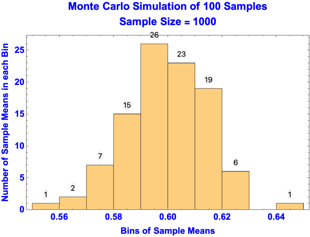
Monte Carlo Simulation of 95% Confidence Level
- A Monte Carlo simulation confirms that the 95% confidence interval = 0.6 ± 0.03 for 1000-member samples.
- In the simulation one hundred 1000-member random samples are taken from the population, with the result that 96 sample means (in red) are in the 0.57-0.63 range.
- 0.559, 0.569, 0.569, 0.576, 0.576, 0.576, 0.578, 0.578, 0.578, 0.579,0.582, 0.583, 0.583, 0.583, 0.584, 0.585, 0.586, 0.586, 0.586, 0.586,0.586, 0.587, 0.587, 0.587, 0.589, 0.59, 0.591, 0.591, 0.592, 0.592,0.592, 0.592, 0.593, 0.593, 0.593, 0.594, 0.595, 0.595, 0.595, 0.595,0.596, 0.596, 0.596, 0.596, 0.597, 0.597, 0.598, 0.598, 0.599, 0.599,0.599, 0.6, 0.6, 0.6, 0.6, 0.6, 0.601, 0.602, 0.602, 0.604, 0.604,0.604, 0.604, 0.604, 0.605, 0.605, 0.605, 0.606, 0.607, 0.607, 0.608,0.608, 0.609, 0.609, 0.61, 0.61, 0.61, 0.61, 0.61, 0.61, 0.611,0.611, 0.611, 0.612, 0.612, 0.614, 0.614, 0.615, 0.615, 0.616, 0.616,0.616, 0.618, 0.624, 0.625, 0.625, 0.626, 0.626, 0.627, 0.642
- In the histogram of the 100 simulated sample means, there is:
- 1 sample mean in the 0.55-0.56 range
- 2 in the 0.56-0.57 range
- 96 in the 0.57-0.63 range
- 1 in the 0.64-0.65 range
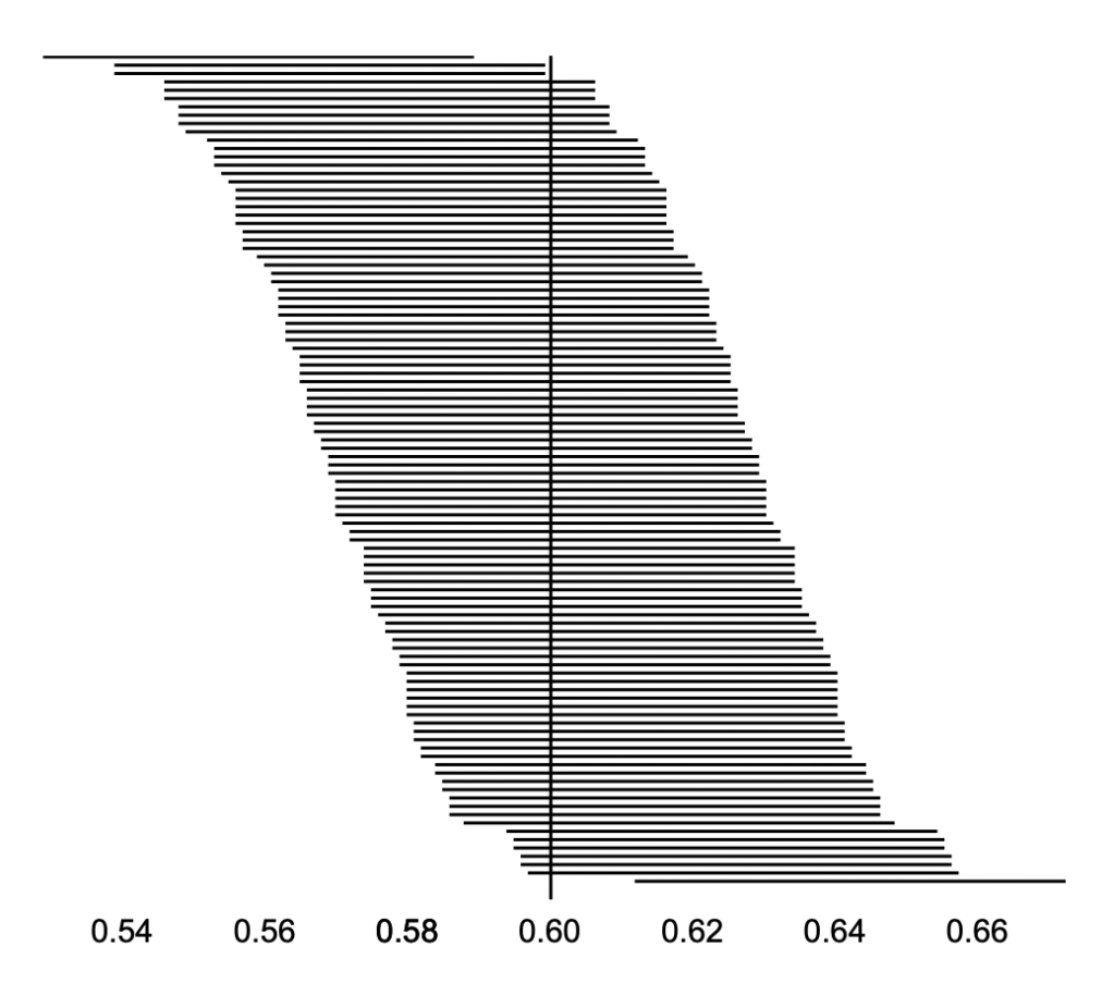
- In the graph below:
- The horizontal lines represent intervals of the sample means, plus and minus the margin of error.
- The top line, for example, represents the sample means 0.559, extending from 0.529 to 0.589
- The vertical line is the population mean, 0.6
- The horizontal lines represent intervals of the sample means, plus and minus the margin of error.
- 96 sample means “cover” the population mean.
- Four don’t:
- Line 1: 0.559±0.03
- Line 2: 0.569±0.03
- Line 3: 0.569±0.03
- Line 100: 0.642±0.03
- Arguments
- objective vs subjective
- inference of population parameter outside and inside statistics
- probability statements in statistics must be testable by repeated experiments, as they are in physics (Quantum Mechanics, for example).
Bayesian Estimation
- Bayes Theorem for n competing hypotheses Hi
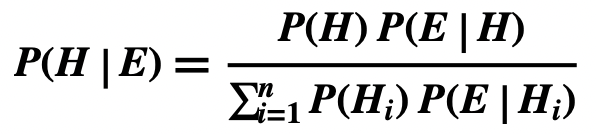
- where H and E are propositions
- View Bayes Theorem
- Bayesian Estimation uses a variant of this form, replacing H with random variable θ, E with y, and the sum of His with the integral of θ.
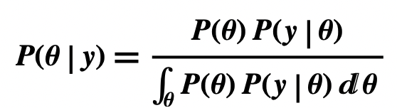
- where
- θ is a random variable for a proportion of the population, for instance, the proportion of the population approving the president’s job performance.
- P(θ) is its prior probability, that is, the probability of θ before data is considered
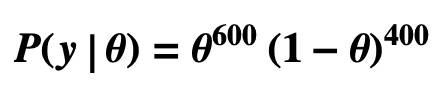
- y is the data, for example a random sample consisting 600 ones and 400 zeros, with ones representing approval of the president’s job performance and zeros representing disapproval.
- y|θ is a random variable for the data y given θ, and P(y|θ) its likelihood.
- θ|y is a random variable for θ given the data y, and P(θ|y) its posterior probability.
- the denominator is the integral of P(θ)P(y|θ) for all values of θ.
- θ is a random variable for a proportion of the population, for instance, the proportion of the population approving the president’s job performance.
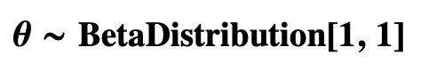
- The result of the calculation below:
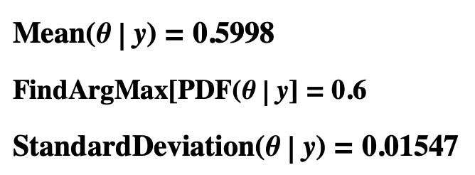
- The expectation of θ|y is 0.5998 and its standard deviation 0.01547.
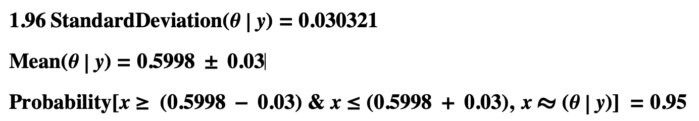
- At the 95% credible level, the mean is 0.5998 ± 0.03
Calculation using Bayes Theorem
- Bayes Theorem with random variable θ = the proportion of the population who approve of the president’s job performance
- Numerator
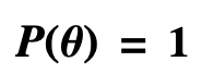
- Uniform Prior Probability of θ = P(θ)
- Likelihood of Data y given θ = P(y|θ)
- Uniform Prior Probability of θ = P(θ)
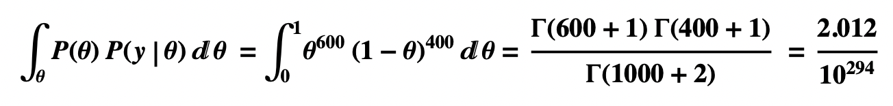
- Denominator, the Integral of P(θ) P(y|θ) for all values of θ
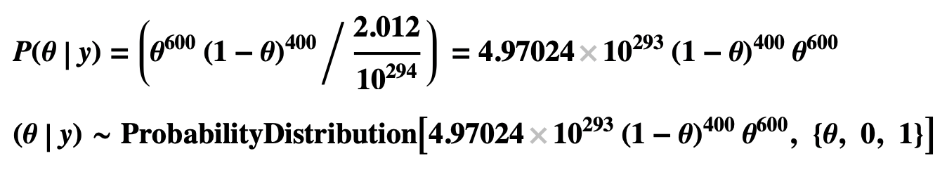
- Posterior Probability of θ = P(θ|y)
- Mean, Mode, and Standard Deviation of Probability Distribution θ|y
- 95% Credible Interval for θ|y
Shortcut Calculation using Beta Distribution
- Uniform Prior Probability of θ
- Posterior Probability of θ|y
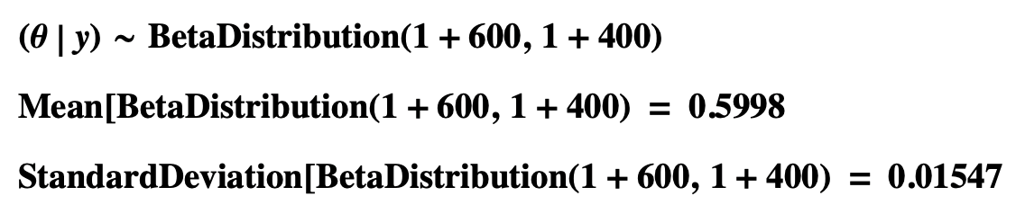
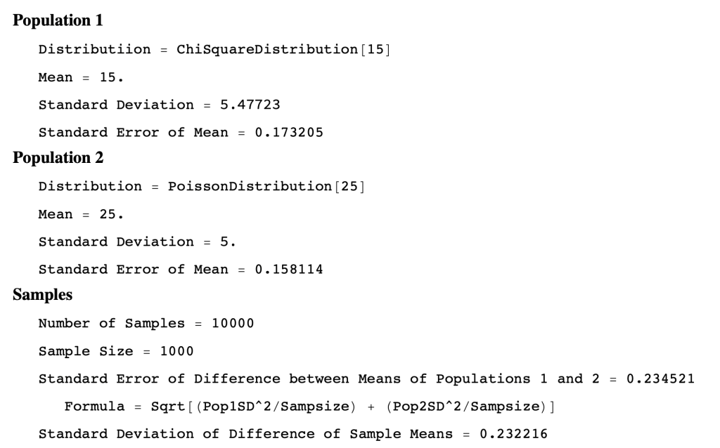
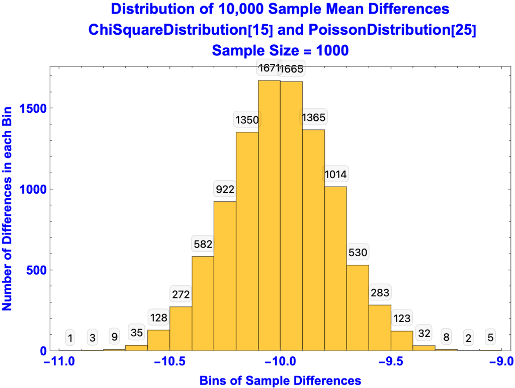
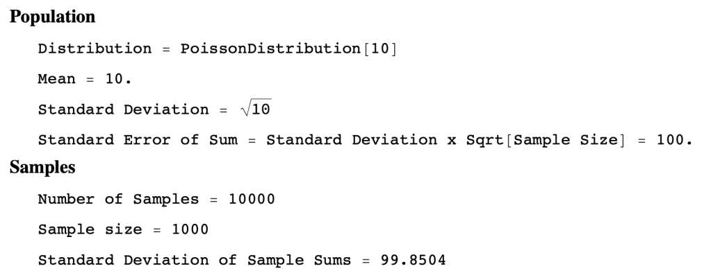
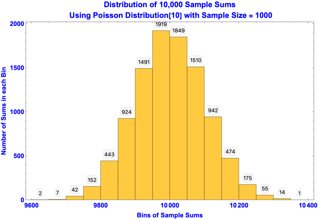
Comparison of Standard Error with Standard Deviation of Simulated Samples
Standard Error of Sample Means
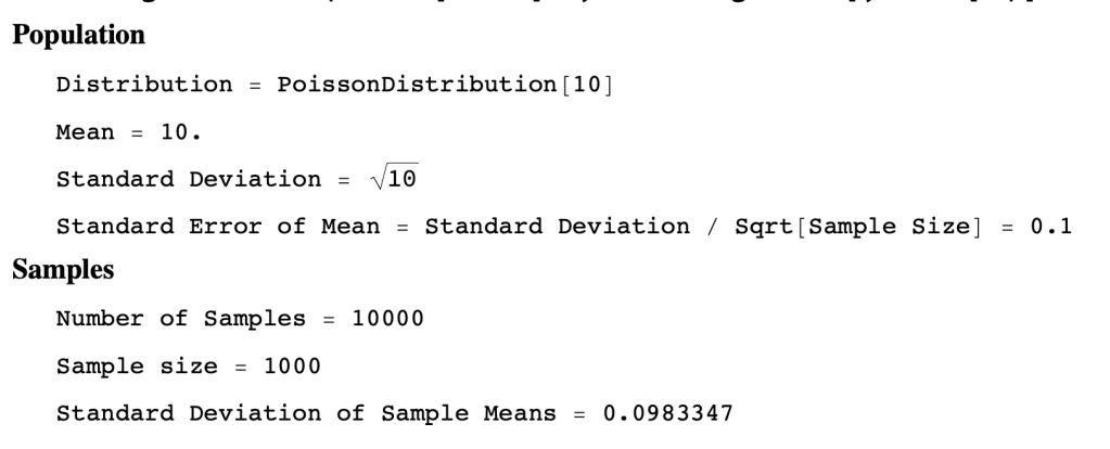

Standard Error of Sample Proportions

Standard Error of Sample Sums
Standard Error of Difference of Sample Means