Postulates and Prediction

Back to Quantum Mechanics

Outline

Prediction in Classical and Quantum Physics
Postulates of Classical Mechanics
1. How Classical Mechanics Predicts the Behavior of the Bowling Balls
Postulates of Orthodox Quantum Mechanics
1. How Quantum Mechanics Predicts Vertical Spin
What Predictions in Classical and Quantum Mechanics Look Like
1. Prediction in Classical Mechanics
2. Prediction in Quantum Mechanics
Addendum: Mathematics of Prediction of Vertical Spin

Prediction in Classical and Quantum Physics

Prediction in Classical Physics, an Example

Suppose that two 16 pound bowling balls are at rest 10 meters apart (center to center) in otherwise empty intergalactic space. The diameter of the bowling balls is 8.595 inches. Using Newton’s Law of Motion (F = MA) and his Law of Gravitation (F = Gm₁m₂/d²), Classical Mechanics predicts the bowling balls will collide in 13 days, 1 hour, 3 minutes, and 38 seconds.
View Bowling Ball Interactive
I did the calculation using Runge-Kutta numerical methods.
The calculation can also be done analytically, using this formula for the time until “center-to-center” impact:

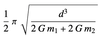
Prediction in Quantum Mechanics, an Example

In addition to mass and electrical charge an electron has an intrinsic spin, which makes an electron a tiny magnet with north and south poles. When the vertical spin of an electron is measured, the result is either spin-up or spin-down. When the horizontal spin of an electron is measured, the result is either spin-left or spin-right.
Suppose that the spin of an electron is prepared so its horizontal spin is spin-right. If the horizontal spin is measured QM not surprisingly predicts the outcome will be spin-right. Which is what happens. But if its vertical spin is measured QM predicts that the outcome will either be spin-up with probability 1/2 or spin-down with probability 1/2. That’s what’s observed when the experiment is done thousands of times.

How the Predictions Differ

The predictions of CM and QM differ in two fundamental ways.
The most radical difference is that CM predicts what happens in a physical system while QM predicts only the outcome of a measurement. Thus, CM tracks the bowling balls as they accelerate toward each other for the 13 days before they collide. But QM says nothing about the electron’s spin between its preparation in a spin-up state and the measurement of its horizontal spin.
The second difference is that CM’s predictions are categorical while those of QM are fundamentally probabilistic.

Postulates of Classical Mechanics

In its most basic form, the postulates of Classical Mechanics are Newton’s Laws of Motion:
- F = MA
  - The net force on an object (in a certain direction) equals the mass of the object times its acceleration (in that direction).
- Third Law
  - For every force on an object (in a certain direction) there’s an equal force on some object or other (in the opposite direction).
    - Newton’s Law of Gravitation, for example, ascribes equal and opposite forces to any pair of objects.
- (Newton’s Law of Inertia is implied by F = MA when F = 0.)

How Classical Mechanics Predicts the Behavior of the Bowling Balls

The postulates of Classical Mechanics predict the collision of the bowling balls by tracking their location through time.
The tracking process is essentially a loop through moments of time:
- Compute the force on each bowling ball at a given moment using Newton’s Law of Gravitation.
- Compute the acceleration of each bowling ball at that moment per A = F / M.
- Compute the location and velocity of each bowling ball at the next moment.
- Repeat for next moment.

Postulates of Orthodox Quantum Mechanics

State Vector Representation
- The state of a physical system at a given time is represented by vector |ψ⟩ in a complex Hilbert space having either a finite or infinite number of dimensions.
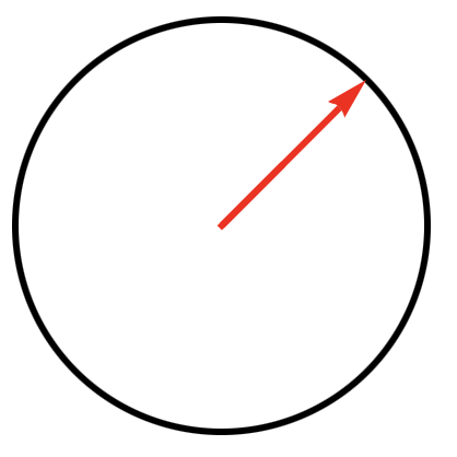
  - The state vector can be visualized (in two-dimensional space) as an arrow from the center of a circle to its edge. Examples:
Observable/Operator Representation
- Every measurable property of a physical system (called an observable) is represented by a linear, Hermitian operator on a Hilbert space. Observables include location, momentum, angular momentum, spin, energy, kinetic energy. Operators are also used to represent measuring devices.
  - An operator applied to a vector generates a new vector.
  - Operators have eigenvalues and eigenvectors defined by equations of the form:
    - Operator ・ |eigenvector⟩ = eigenvalue |eigenvector⟩
      - where the dot is matrix multiplication
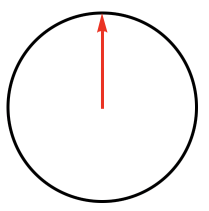
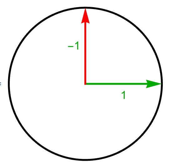
  - An operator (in two-dimensional space) can be depicted as two radius arrows at right angles:
  - The arrows represent the operator’s eigenvectors and the numerals their eigenvalues.
Time Evolution of the State Vector
- As long as no observable of the system is measured, the state vector |ψ⟩ evolves continuously and deterministically according to the Schrödinger Equation, ℏ ∂|Ψ⟩/∂t = -iH|Ψ⟩, where operator H is the Hamiltonian of the system.
  - The Hamiltonian of a system represents its total energy.
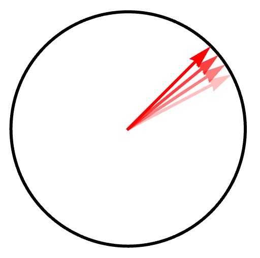
- The time evolution of the state vector (in a two-dimensional space) can be visualized by the red arrow rotating within the circle.
Prediction of a Measurement
- If the system is in state |ψ⟩ and an observable with operator M is measured, the probability of outcome λ is |⟨Ψ|λ⟩|², where
  - λ is an eigenvalue of M,
  - |λ⟩ is its corresponding eigenvector,
  - ⟨Ψ|λ⟩ is the inner product of Ψ and λ.
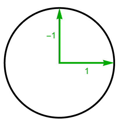
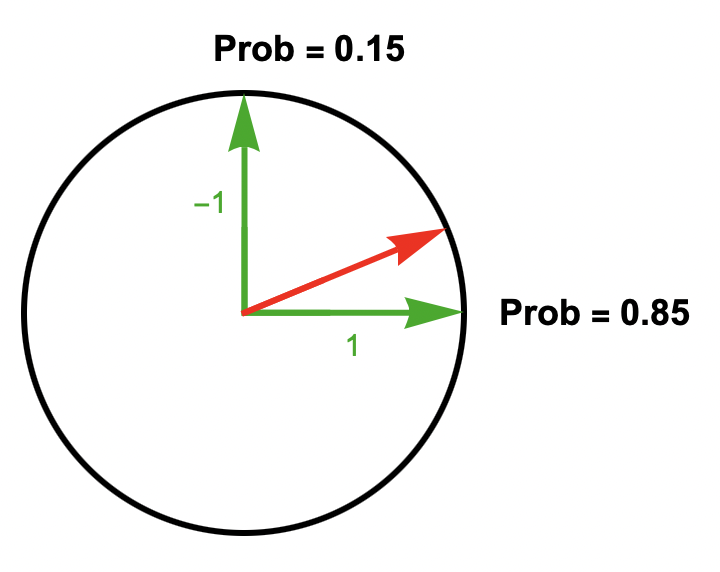
- A prediction (in a two-dimensional space) can be depicted by combining diagrams of the state vector and operator:
- The diagram represents the prediction that the outcome of the measurement is either 1 (with probability 0.85) or -1 (with probability 0.15).
  - (The smaller the angle between the state vector and an eigenvector, the greater the probability of the eigenvector’s eigenvalue.)
Collapse of the State Vector
- If an observable (with operator M) is measured with outcome λ, the state vector |ψ⟩ of the system immediately after the measurement is the eigenvector of M with eigenvalue λ.
  - Right after a measuring an observable (in a two-dimensional space) the system will be in one or the other of these states:

How Quantum Mechanics Predicts Vertical Spin

The operators for horizontal and vertical spin look like this.
The operator for horizontal spin has eigenvectors |r> (spin-right) with eigenvalue +1 and |l> (spin-left) with eigenvalue -1.
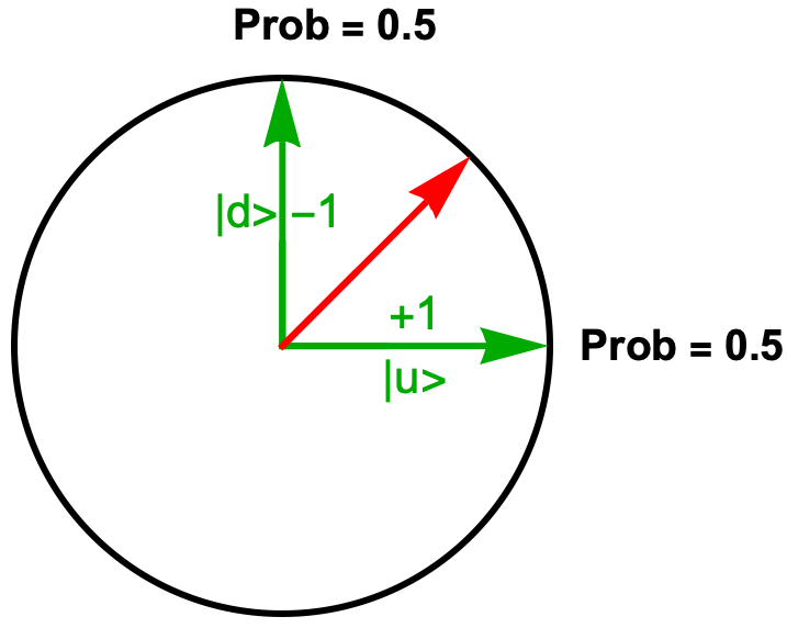
The operator for vertical spin has eigenvectors |u> (spin-up) with eigenvalue +1 and |d> (spin-down) with eigenvalue -1.
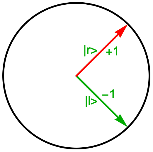
To prepare the horizontal spin of an electron in the spin-right state, you measure the horizontal spin until the outcome is +1. The resulting state vector is |r>, per the Collapse Postulate. So the system looks like this:
With no forces on the electron, the state vector remains in this position until a measurement takes place, per the Time Evolution Postulate. Given the location of the state vector, the Prediction Postulate generates the following prediction for the outcome of measuring vertical spin:

What Predictions in Classical and Quantum Mechanics Look Like

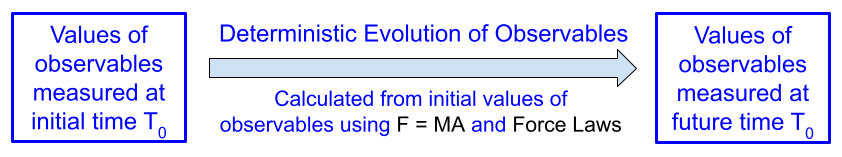
Prediction in Classical Mechanics

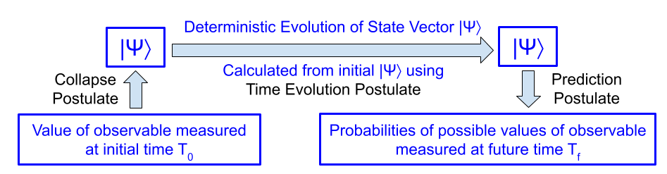
Prediction in Quantum Mechanics

Addendum: Mathematics of Prediction of Vertical Spin

Spin operators are expressed mathematically as two-dimensional matrices called Pauli matrices.
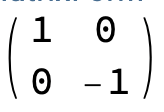
Matrices for σ_x and σ_z, the horizontal and vertical spin operators, are:
- σ_x =
- σ_z =

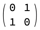
The eigen-equations, eigenvectors, and eigenvalues for σ_x are:
- σ_x ・ lr> = 1 lr>
  - where lr> = {1/√2, 1/√2}
  - where the dot is matrix multiplication
- σ_x ・ lr> = -1 ll>
  - where ll> = {1/√2, -1/√2}
  - where the dot is matrix multiplication.

The eigen-equations, eigenvectors, and eigenvalues for σ_z are:
- σ_z ・ lu> = 1 lu>
  - where lu> = {1, 0}
  - where the dot is matrix multiplication
- σ_z ・ ld> = -1 ld>
  - where ld> = {0, 1}
  - where the dot is matrix multiplication.

Finally, the probabilities that lr> collapses into |u> and |d> are:
- |<r|u>|² = 1/2
  - where <r|u> = Conjugate of |r> ・|u> = 1/√2
  - so |<r|u>|² = (1/√2)² = 1/2
- |<r|d>|² = 1/2
  - where <r|u> = Conjugate of |r> ・ |d> = 1/√2
  - so |<r|d>|² = (1/√2)² = 1/2.