Contents
- Data, Variables, and Values
- Categorical, Ordinal, Interval, and Ratio Variables
- Statistics of a Single Variable
- Data Visualization
Data, Variables, and Values
- Descriptive Statistics uses mathematics and visualization to throw light on collected data.
- Data are recorded facts about entities and their properties, i.e. the values of variables.
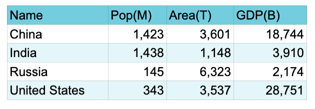
- A dataset is an organized collection of data, typically arranged as a table with rows (records) and columns.
- For example
- The variables of the dataset are the column headings: Name, Population (in millions), Area (in thousands of square miles) and GDP (in billions of dollars). The variable Name identifies the entity (country) which possesses the specified values of the other variables.
- The values of the variable Population are: 1423, 1438, 145, and 343. The values of Area are: 3601, 1148, 6323, and 3537. And the values of GDP are: 18744, 3910, 2174, and 28751.
Categorical, Ordinal, Interval, and Ratio Variables
- Mathematical relations and operations apply to variables in different degrees:
- Categorical: x = y and x ≠ y
- Ordinal: x > y and x < y (in addition to x = y and x ≠ y)
- Interval: x + y and x – y (in addition to x > y and x < y and x = y and x ≠ y)
- Ratio; x ・ y and x / y (in addition to x + y and x – y and x > y and x < y and x = y and x ≠ y).
Categorical (Qualitative, Nominal) Variables
- The values of categorical variables are labels with no meaningful order. For example:
- Eye color: blue, brown, green
- Blood type: A, B, AB, O
- Car brand: Toyota, Ford, Honda
- Numbers are sometimes used in place of alphanumeric labels, e.g. 1 = employed and 0 = unemployed. Such numbers are merely numerals used as labels.
- The only mathematical relations that meaningfully apply to categorical variables are: x = y and x ≠ y, indicating merely that entities have the same or different values of a categorical variable.
- A special kind of categorical variable — identifiers — denote entities. Thus the identifier “China” denotes the entity China, which possesses values of other variables, such as population, area and GDP. Other countries may have the same population or area or GDP but not the same identifier.
Ordinal Variables
- Ordinal variables are those for which x > y and x < y are meaningful (in addition to x = y and x ≠ y). But for which x + y and x – y are meaningless. That is, ordinal variables define levels such that one entity can have a higher or lower level of a variable than another entity. But ordinal variables don’t support the fundamental operations of arithmetic (addition, subtraction, multiplication, division).
- Suppose, for example, that the values of Education Level are the numbers 1 to 6 such that:
- 1 = No high school diploma
- 2 = High school diploma or GED.
- 3 = Some college credits earned but no degree.
- 4 = Associate degree
- 5 = Bachelor’s Degree
- 6 = Master’s, doctorate, or professional degree
- So, if Amy has educational level x and Mike educational level y, then if x > y Amy has more formal education than Mike.
- But adding educational levels makes no sense. The arithmetic fact that 1 + 2 + 3 = 6 is meaningless when applied to education levels. The problem is that defining education levels does not thereby define “educational units” so that, for example, level 1 = 5 units, level 2 = 10 units, and so on. Addition and subtraction without units make no sense.
Interval Variables
- Interval variables are those for which x + y and x – y are meaningful (in addition to x > y and x < y and x = y and x ≠ y). But for which x ・ y and x / y are meaningless. That is, interval variables define units that can be added and subtracted but not multiplied and divided.
- Consider year-of-birth. If Amy is born in year x and Mike in year y, then:
- If x > y, Amy is younger than Mike.
- If x – y = 2, Amy is two years younger than Mike.
- But x / y = 2 does not mean that Amy is twice as old as Mike.
- Other examples are temperature in Fahrenheit or Celsius, IQ scores, and dates.
Ratio Variables
- Ratio variables are those for which x ・ y and x / y are meaningful (in addition to x + y and x – y) . That is, ratio variables define units that can be multiplied and divided as well as added and subtracted. They also have a “true zero,” denoting a complete lack of the variable.
- Consider a person’s age in years. Suppose Amy is x years of age and Mike is y years of age. Then:
- If x > y, Amy is older than Mike.
- If x – y = 2, Amy is two years older than Mike.
- If x / y = 2, Amy is twice as old as Mike.
- If x = 1, Amy is one year old.
- If x = 1/365, Amy is one day old.
- If x = 0 Amy has no age.
- Other examples are weight, height, income, distance, duration of time, and temperature in Kelvin.
Statistics of a Single Variable
Dataset
- Contents: Life expectancies (at birth) of 233 countries.
- Source: Wolfram Country Data
- Sample data items:
- 80.626, 82.479, 72.15, 69.887, 68.002, 78.5, 64.045, 82.784, 73.082, 74.8
- Variable Type: Ratio
Mean and Standard Deviation
- The mean of the dataset is 73.91.
- That is, the average life expectancy is 73.91 years.
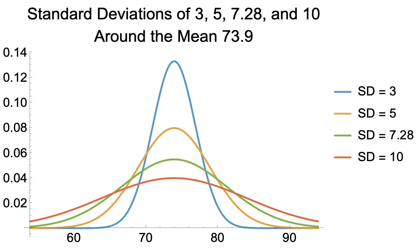
- The standard deviation is 7.28.
- The standard deviation of 7.28 is a measure of the spread of life expectancies around the mean of 73.91. Here’s what a standard deviation of 7.28 looks like, compared to standard deviations of of 3, 5, and 10 (assuming a normal distribution):
- The standard deviation is something like the average distance of data values from the mean. But not exactly. The exact average distance from the mean is the Mean Absolute Deviation, which is 5.88 for the dataset of life expectancies. MAD is easily calculated and understood. Thus, for example, the MAD of the numbers {2, 4, 6}, is ((4 – 2) + (4 – 4) + (6 – 4)) / 3 = 4/3. Statisticians use the standard deviation rather than MAD, however, for theoretical reasons (in particular because of the Central Limit Theorem).
- Mathematically, the standard deviation is the square root of the variance. The variance in turn is the sum of the square deviations of data values from the mean, divided by the number of values minus 1. So for the numbers {2, 4, 6}:
- the sum of square deviations = (4 – 2)2 + (4 – 4)2 + (6 – 4)2 = 8
- the variance = 8 / (3 – 1) = 4
- the standard deviation = √4 = 2.
- The standard deviation of 7.28 is a measure of the spread of life expectancies around the mean of 73.91. Here’s what a standard deviation of 7.28 looks like, compared to standard deviations of of 3, 5, and 10 (assuming a normal distribution):
Order Statistics
- Order statistics, calculated on a sorted dataset, are dividing lines between lower and higher data values. The primary order statistics for the life expectancies dataset are:
- Minimum = 53.68
- Quartiles = {69.77, 75.22, 79.55}
- Median = 75.22
- Maximum = 89.4
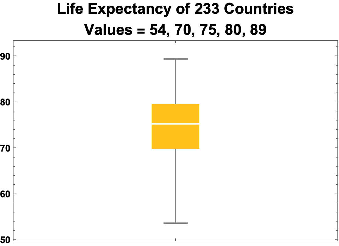
- A box-and-whisker chart depicts the statistics:
-
- Key:
- Minimum (54) is the lower whisker
- First Quartile (70) is the bottom edge of the box
- Median (75) is the white line through the box
- Third Quartile (80) is the top edge of the box
- Maximum (89) is the top whisker.
- The idea underlying order statistics is that of a percentile (or quantile).
- The nth percentile of a dataset is the data value P such that n percent of data items have values less than P and the rest have values greater than P.
- Thus for the life expectancies:
- The median of 75.22 (the 50th percentile) is the dividing line between 116 lower life expectancies (50% of the total 233) and 117 higher expectancies (50% of the total).
- The third quartile of 79.55 (the 75th percentile) is the dividing line between 175 lower life expectancies (75%) and 58 higher expectancies (25%).
- The maximum of 89.4 (the 100th percentile) is the dividing line between 233 lower life expectancies (100%) and 0 higher expectancies (0%).
- Note: There are different ways of drawing the dividing lines. For example, the algorithm I’m using yields 79.55 for the 75th percentile. Other algorithms yield 79.5248, 79.526 and 79.558.
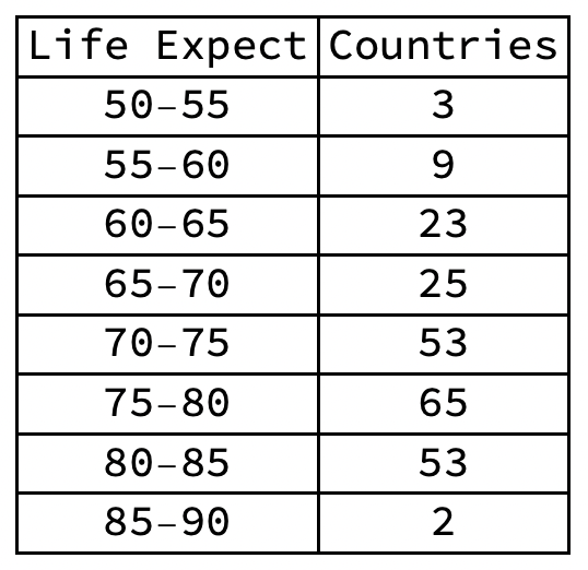
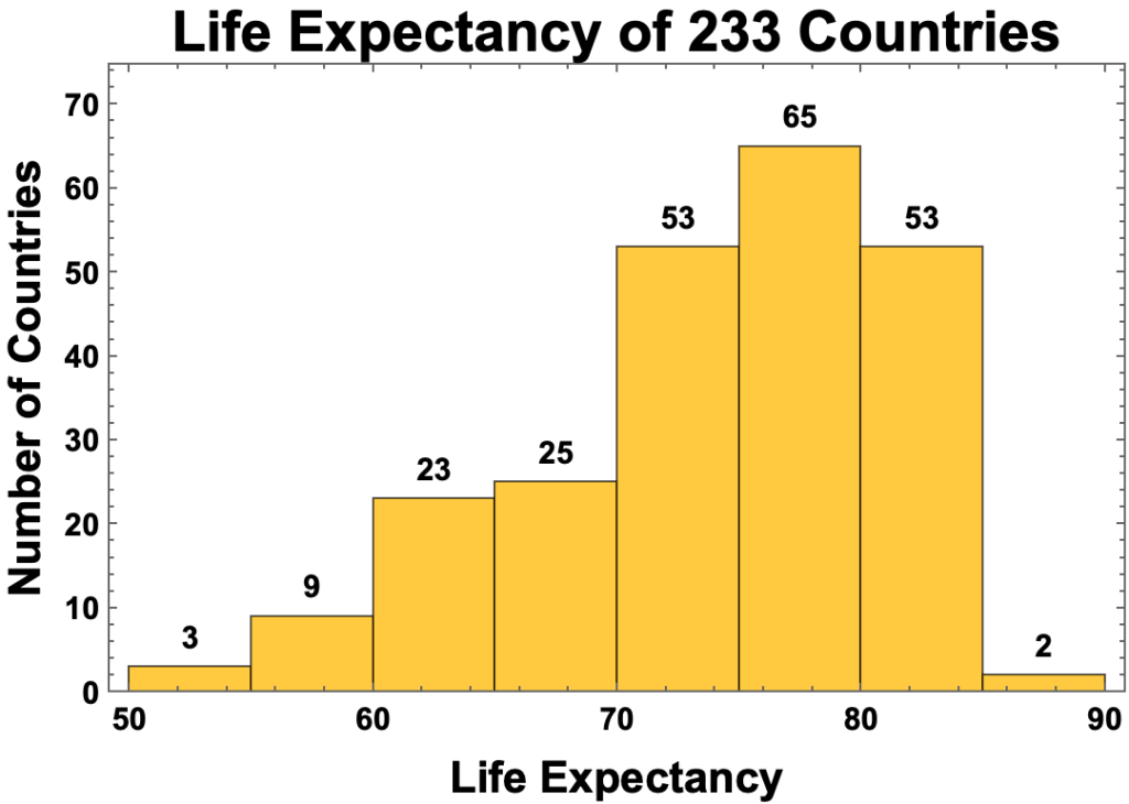
Frequency Distributions and Histograms
- The best tools for getting a feel for the data of a single variable are the frequency distribution and its graphical representation, the histogram.
- Frequency distributions and histograms, on the one hand, and percentiles and quartiles, on the other, are in a sense inverse operations.
- Both separate the data into bins.
- But percentiles and quartiles define the size of bins first and then calculate the data values dividing them.
- Frequency distributions and histograms, by contrast, first define intervals of data values and then calculate the size of bins thus defined.
- For example:
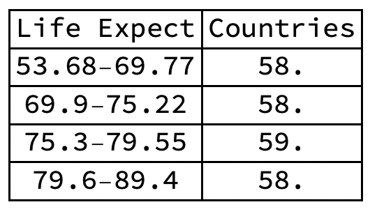

- Quartiles define equal size bins, yielding different intervals of life expectancy.
- Histograms define equal intervals of life expectancy, yielding different size bins.
Data Visualization
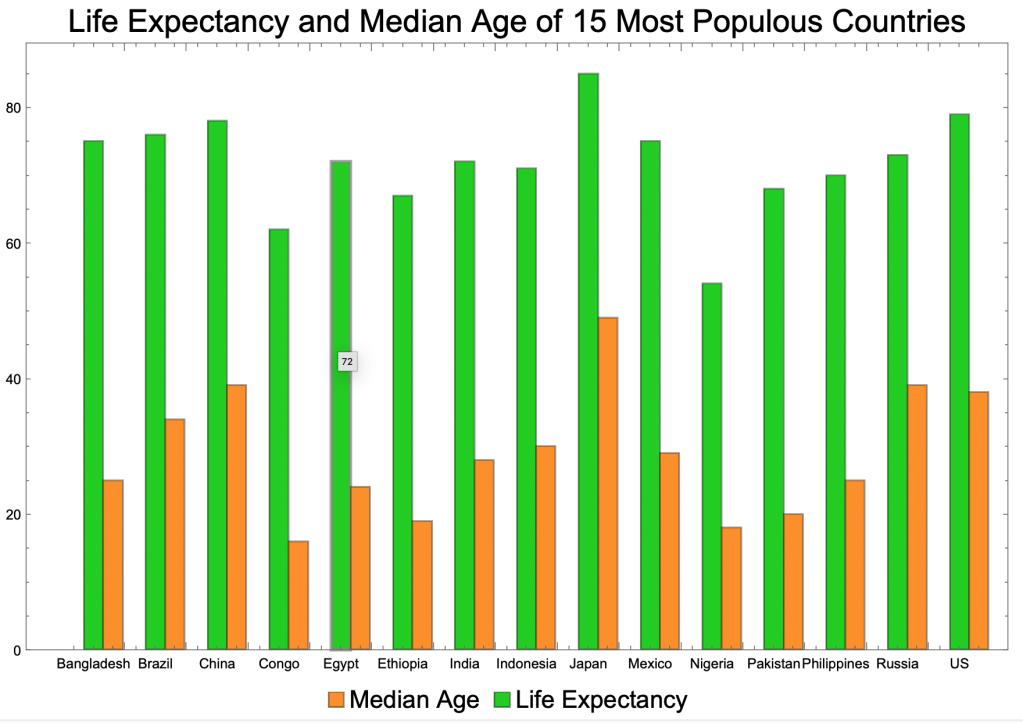
- The natural way of viewing data is in table form, with rows for entities and columns for the values of variables. Here, for example, are sundry statistics for the 15 most populous countries:
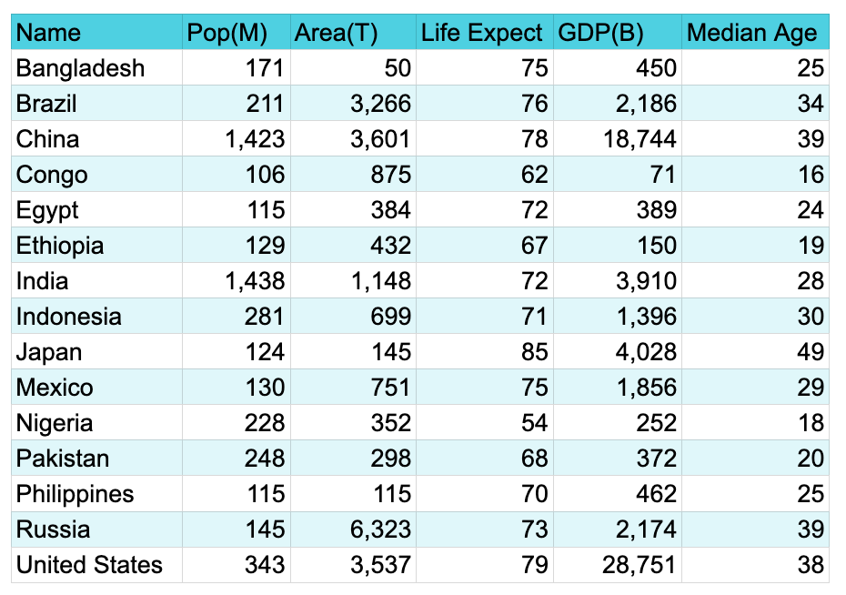
- But the best way to understand data is visually, representing numbers as heights of columns, areas of circles, sectors of circles, points on a coordinate grid, or curves on a coordinate grid. What follows are the main kinds of charts and plots.
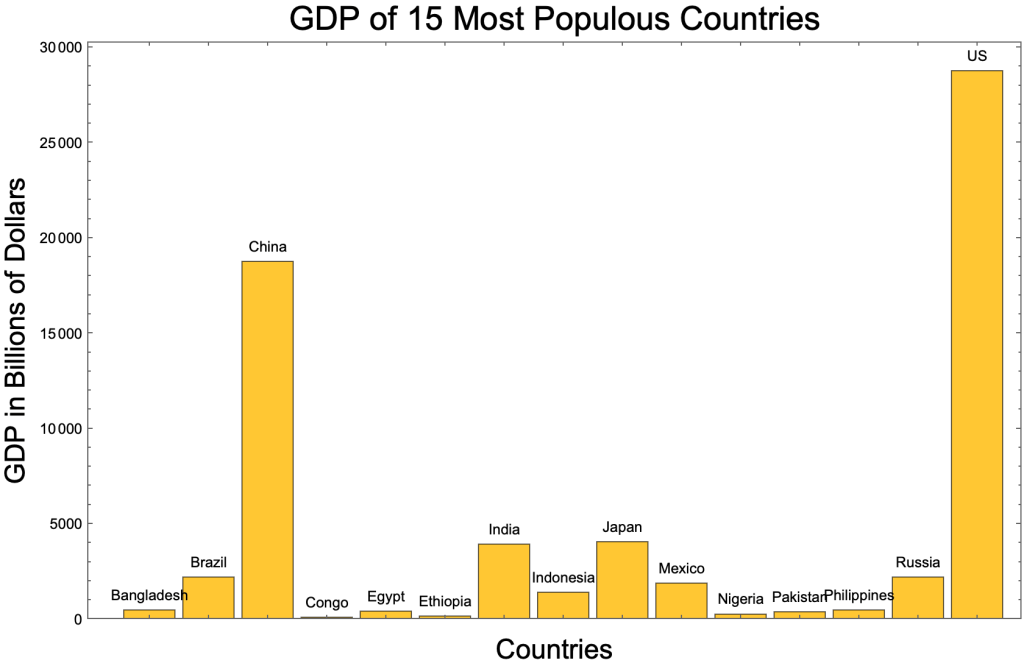
Bar Charts
A bar chart portrays values of a variable as the height of columns.
Grouped bar charts depict multiple variables for the same entity.
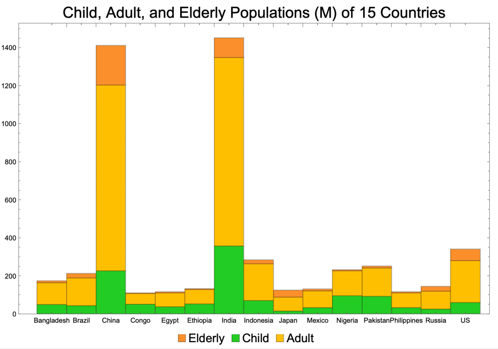
Stacked bar charts represent the components of a variable.
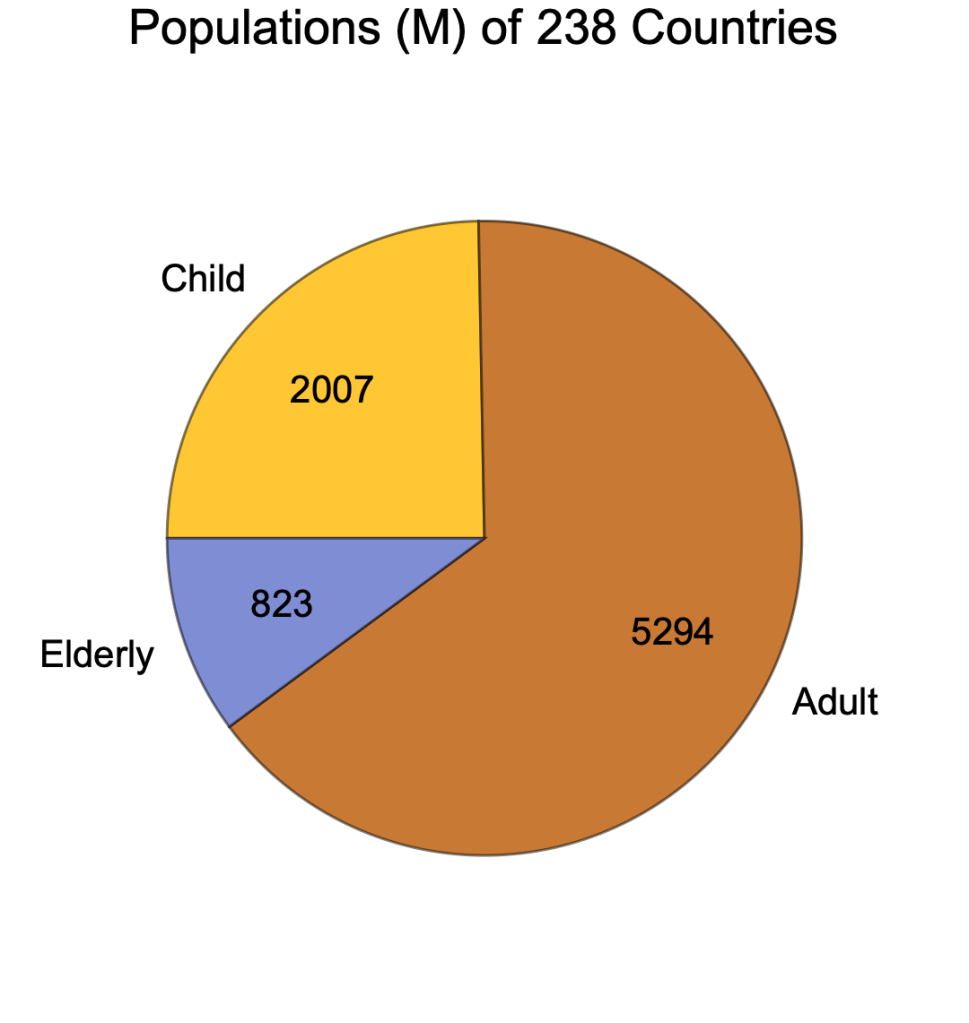
Pie Charts
Pie charts are useful for depicting the components of a variable.
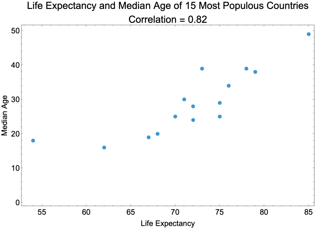
Scatter Plots
Scatter plots are useful for showing correlated variables. The correlation coefficient of 0.82 is on a scale from 0 (no correlation) to 1 (perfect correlation).
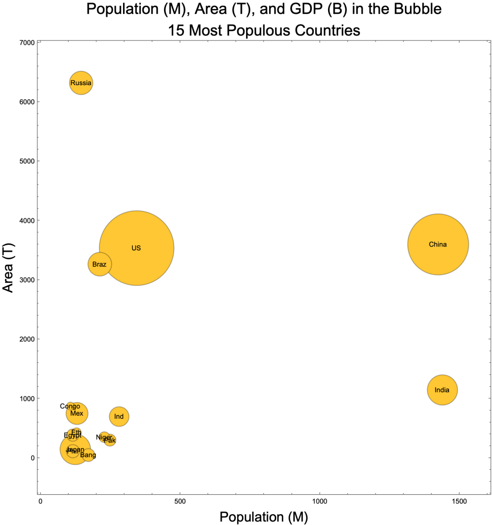
Bubble Charts
Bubble Charts are a clever way of displaying three numeric variables.
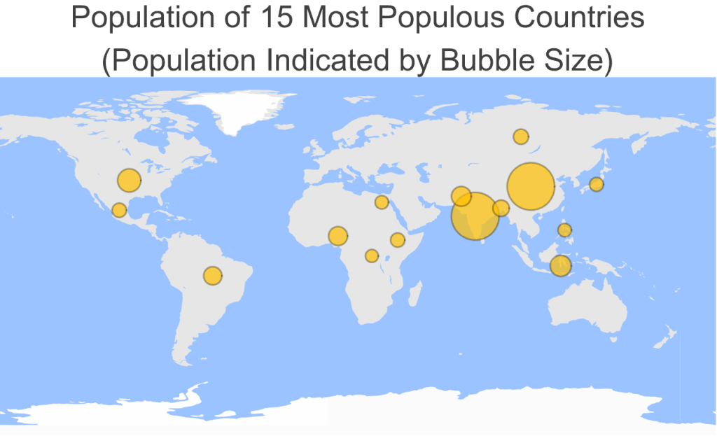
Geo Charts
Geo Charts combine maps and charts, such as this Geo Bubble Chart.
Date Line Plots
Line plots are the classic way to display time series. The Federal Reserve has lots of them at their FRED website. Here’s the monthly trade balance in goods and services from 2016 to 2026 in millions of dollars.
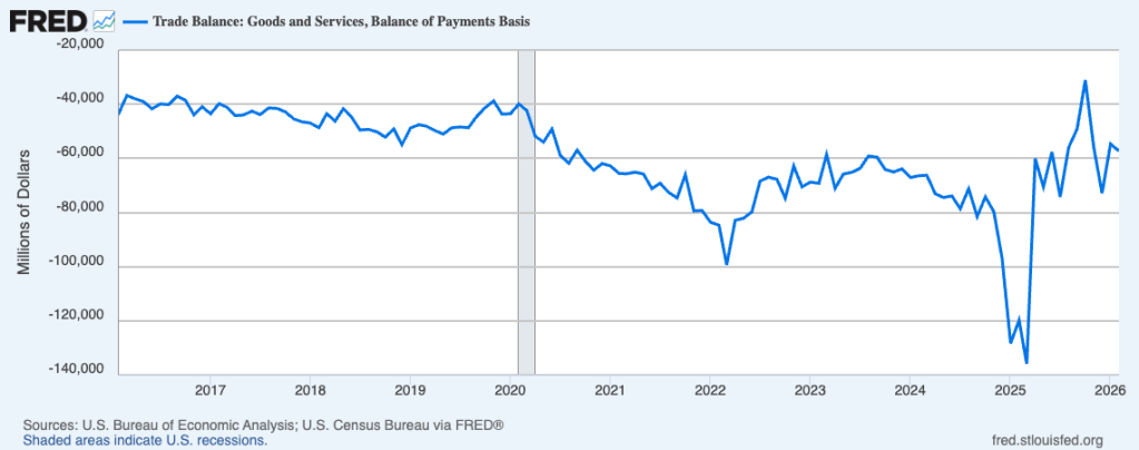
Source: fred.stlouisfed.org/series/BOPGSTB
Addendum: Real World Charts
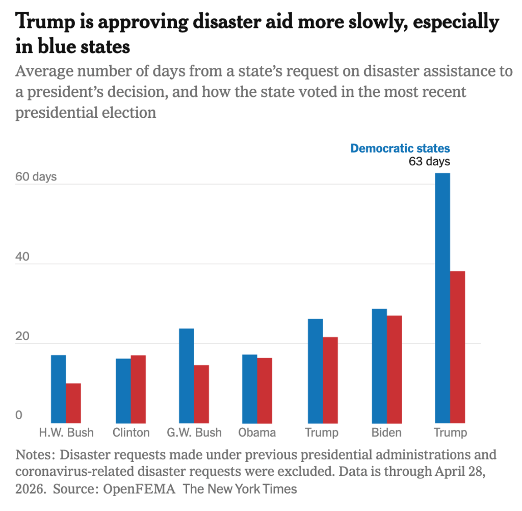
Source: nytimes.com/2026/05/01/climate/fema-disaster-aid-slowdowns.html
