1. Monte Carlo Simulation for Standard Errors of IV and intercept
2. Linear Regression on GDP and IMF
3. NonLinear Regression on GDP and IMF
4. Linear Regression on GDP and Redundant GDP (1/3 times GDP)
5. Linear Regression on GDP, IMF, and Gini
6. NonLinear Regression on GDP, IMF, and Gini
7. Linear Regression on GDP
8. Linear Regression on Random Numbers
9. Linear Regression on

Monte Carlo Simulation for Standard Errors of IV and intercept

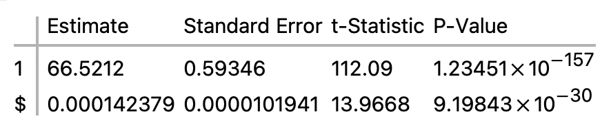
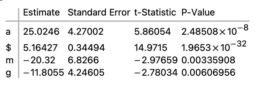
• For the Linear Regression on GDP:
  • The data consists of 167 paired x’s and y’s
  • The regression is: y = 66.5212 + 0.000142379 $
  • The Parameter Table is
    • 

• A Monte Carlo simulation, run with 10,000 iterations, estimated the standard errors as
  • Standard error of intercept = 0.593747
  • Standard error of the variable $ = 0.0000102458

• Monte Carlo simulation for finding the standard error in general
  • Define the population parameter for which the standard error is sought.
  • Loop thousands of times:
    • Take an n-size random sample from the population
    • Compute the statistic of interest for the sample
    • Store the computed sample statistic
  • End Loop
  • The standard error is approximated by the SD of all the computed sample statistics.

• Monte Carlo simulation for finding the standard errors for IV and intercept
  • Define the dataset and regression for which standard errors are sought.
    • We’ll call these the given dataset and the given regression
  • Loop thousands of times:
    • Generate a dataset of random x’s and y’s analogous to the x’s and y’s of the given dataset (this is the tricky part — see below)
    • Do a regression on the analogous dataset
    • Store the a and b coefficients of the regression equation
  • End Loop
  • Calculate the SD of all the a coefficients — that approximates the standard error of the intercept
  • Calculate the SD of the all b coefficients — that approximates the standard error of the IV

• The Tricky part
  • We want make a dataset of  x’s and y’s relevantly like, but not identical with, the x’s and y’s of the given dataset. 
  • The x’s are easy: Use random numbers from the normal distribution with mean and SD of the given x’s. 
  • The y’s are tricky: A y has to bear approximately the same relation to its paired x as do the given y’s to their paired x’s.
    • First, use the given regression equation, and the random x, to compute a predicted y.
    • Then get a random residual from the normal distribution with mean and SD of the given residuals.
    • The y you want is the predicted y minus the random residual.

• Mathematica Code
  • big$iterations = 10000;
  • bigout = List[];
  • dc = Length[regress[“Data”]];
  • serorig = Sqrt[Total[regress[“FitResiduals”]^2]/(dc-(1+1))];
  • sdforx=Sqrt[N[Total[Table[(regress[“Data”][[i,1]] – Mean[regress[“Data”][[All,1]]])^2,{i,1,dc}]]]/(dc -(1+1))];
  • meanforx =N[Mean[regress[“Data”][[All,1]]]];
  • Do[
    • inside$iterations = dc;
    • sampstat = List[];
    • Do[
      • resrand=RandomVariate[NormalDistribution[0,serorig]];
      • xrand = RandomVariate[NormalDistribution[meanforx, sdforx]];
      • predicty=regress[“Function”][xrand];
      • observedy=predicty-resrand;
      • sampstat =Append[sampstat, {xrand,observedy} ];,
      • {inside$iterations}];
    • sampregress=LinearModelFit[sampstat,x,x];
    • tmpa=sampregress[“ParameterTableEntries”][[1,1]];
    • tmpb=sampregress[“ParameterTableEntries”][[2,1]];
    • bigout =Append[bigout, {tmpa,tmpb} ];,
    • {big$iterations}]
  • regress[“ParameterTable”]
  • StandardDeviation[bigout[[All,1]]]
  • StandardDeviation[bigout[[All,2]]]

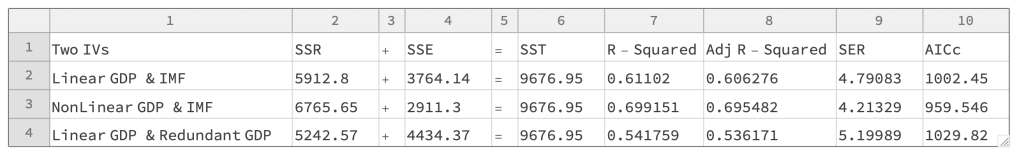
Linear Regression on GDP and IMF

• Regression Equation; y = 68.4357 – 40.3304 m + 0.000124256 $
• DataPoints = 167
• NbrofIVs = 2
• Sum of Squares Equation: 5912.8 + 3764.14 = 9676.95
  • SSR + SSE = SST, where SSR, SSE, and SST are the sums of squares for
    • predicted y’s
    • residuals
    • observed y’s
• Standard Error of the Regression = 4.79083
  • = √(SSE / (Datapoints – (NbrofIVs + 1)))
• R-Squared = 0.61102
  • = SSR / SST
• Adjusted R-Squared = 0.606276
• AICc = 1002.45

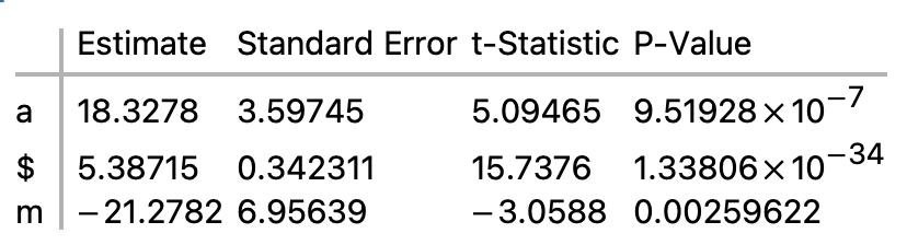
NonLinear Regression on GDP and IMF

• Regression Equation; y = 18.3278 – 21.2782 y + 5.38715 Log[x]
• DataPoints = 167
• NbrofIVs = 2
• Sum of Squares Equation: 6765.65 + 2911.3 = 9676.95
  • SSR + SSE = SST, where SSR, SSE, and SST are the sums of squares for
    • predicted y’s
    • residuals
    • observed y’s
• Standard Error of the Regression = 4.21329
  • = √(SSE / (Datapoints – (NbrofIVs + 1)))
• R-Squared = 0.699151
  • = SSR / SST
• Adjusted R-Squared = 0.695482
• AICc = 959.546

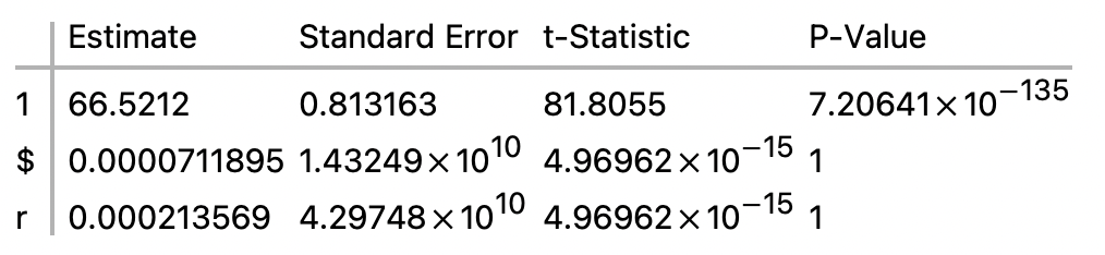
Linear Regression on GDP and Redundant GDP (1/3 times GDP)

• Regression Equation; y = 66.5212 + 0.000213569 r + 0.0000711895 $
• DataPoints = 167
• NbrofIVs = 2
• Sum of Squares Equation: 5242.57 + 4434.37 = 9676.95
  • SSR + SSE = SST, where SSR, SSE, and SST are the sums of squares for
    • predicted y’s
    • residuals
    • observed y’s
• Standard Error of the Regression = 5.19989
  • = √(SSE / (Datapoints – (NbrofIVs + 1)))
• R-Squared = 0.541759
  • = SSR / SST
• Adjusted R-Squared = 0.536171
• AICc = 1029.82

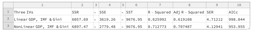
Linear Regression on GDP, IMF, and Gini

• Regression Equation; y = 73.3606 – 12.435 g – 38.764 m + 0.00011775 $
• DataPoints = 167
• NbrofIVs = 3
• Sum of Squares Equation: 6057.69 + 3619.26 = 9676.95
  • SSR + SSE = SST, where SSR, SSE, and SST are the sums of squares for
    • predicted y’s
    • residuals
    • observed y’s
• Standard Error of the Regression = 4.71212
  • = √(SSE / (Datapoints – (NbrofIVs + 1)))
• R-Squared = 0.625992
  • = SSR / SST
• Adjusted R-Squared = 0.619108
• AICc = 998.044

NonLinear Regression on GDP, IMF, and Gini

• Regression Equation; y = 25.0246 – 20.32 y – 11.8055 z + 5.16427 Log[x]
• DataPoints = 167
• NbrofIVs = 3
• Sum of Squares Equation: 6897.47 + 2779.48 = 9676.95
  • SSR + SSE = SST, where SSR, SSE, and SST are the sums of squares for
    • predicted y’s
    • residuals
    • observed y’s
• Standard Error of the Regression = 4.12941
  • = Sqrt(SSE / (Datapoints – (NbrofIVs + 1)))
• R-Squared = 0.712773
  • = SSR / SST
• Adjusted R-Squared = 0.707487
• AICc = 953.955

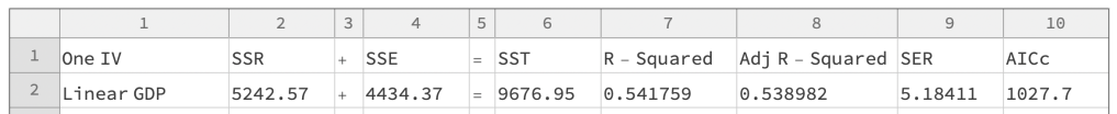
Linear Regression on GDP

• Linear Regression on GDP
• Regression Equation: y = 66.5212 + 0.000142379 x
• DataPoints = 167 and Independent Variables = 1
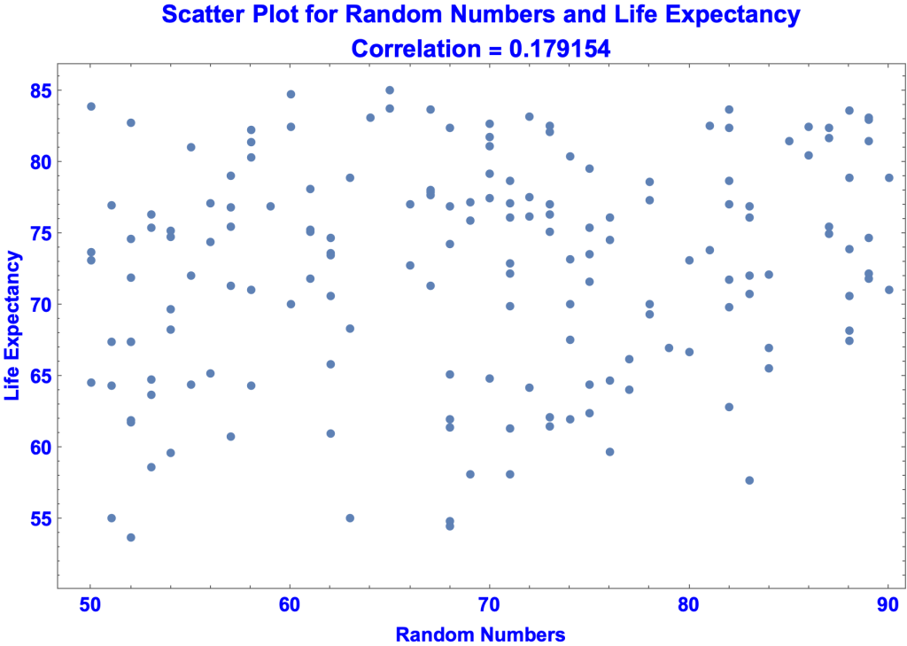
• Correlation between GDP and LE = 0.736
• Sum of Squares Equation: 5242.57 + 4434.37 = 9676.95
• R-Squared = 0.541759 and Adjusted R-Squared = 0.538982
• Standard Error of the Regression = 5.18411
• AICc = 1027.7

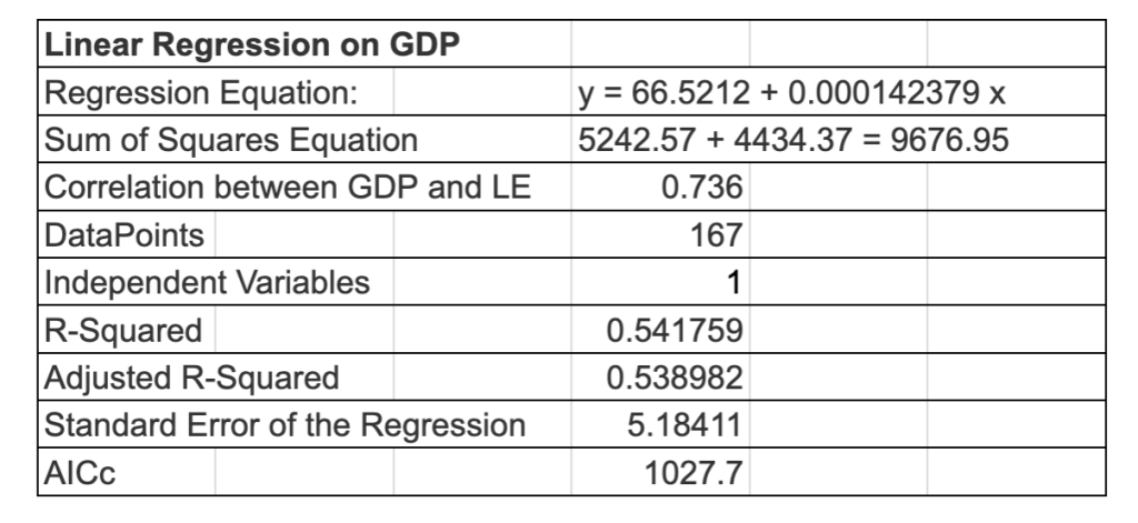
• Analysis
• Correlation
  • Pretty good correlation between GDP and Life Expectancy, 0.736
• Graphs
  • The data curves to the right, suggesting that a nonlinear regression might do better.
• Standard Error of the Regression
  • We’ll see how 5.18411 compares to later regression.
• P-Values for t-Statistics for the standard errors of the coefficients
  • Very high. But that’s assuming that the regression equation is correct.
• R-Squared and Adjusted R-Squared
  • R-Squared is 0.541759, meaning that the regression captures about 54% of the life expectancy scatter. That’s fine, but not great.
• AICc
  • We’ll see how 1027.7 compares to later regression.

Linear Regression on Random Numbers

• Analysis
• Correlation
  • Terrible 0.179154
• Graphs
  • Random dots
• Standard Error of the Regression
  • 7.53431
• P-Values for the t-Statistics for the standard errors of the coefficients
  • 0.02 for x
• R-Squared and Adjusted R-Squared
  • 0.032096 versus SSE / SST = 0.967904
• AICc
  • 1152.57

Linear Regression on

• I’ll evaluate the regressions using
  • Graphs
  • Correlations
  • The following metrics
    • Standard Error of the Regression
    • t-Statistics for the standard errors of the coefficients
    • R-Squared
    • Adjusted R-Squared
    • AICc