Contents
- Regression Analysis
- Simple Linear Regression
- Multiple Linear Regression
- NonLinear Regression
- Evaluating Regressions
- Addendum
Regression Analysis
Regression Equation
- Regression Analysis is a set of procedures for finding and evaluating the simplest equation that most accurately predicts the observed values of a variable from the observed values of other variables.
- The predicted variable, called the dependent variable, is said to be regressed on the independent variables.
- The equation is called the regression equation.
Two Uses
- Prediction
- The regression equation is used to predict unobserved values of the dependent variable from unobserved values of the independent variables.
- Analysis of causal factors
- Regression analysis is used to assess the causal factors that affect a variable.
Simple Linear Regression
Definition
- Simple Linear Regression is regression whose equation has the form y = a + bx where
- y is the dependent variable, the variable to be predicted
- x is the independent variable
- a and b are place-holders for numbers to be filled in by the Least Squares Algorithm.
- Suppose data is collected for variables x and y.
- data{x,y} ={{51,55},{100,68},{63,60},{52,40},{67,45},{42,49},{81,62},{70,56},{108,93},{90,76}}
- The variables are correlated, meaning that they tend to vary together, in the same or opposite directions.
- The correlation coefficient, which goes from -1 to +1, is a measure of the degree of correlation, in this case 0.853422
- View page on Correlation
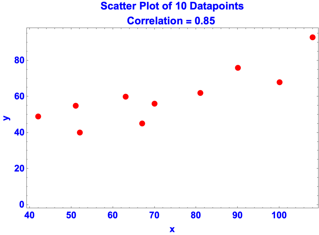
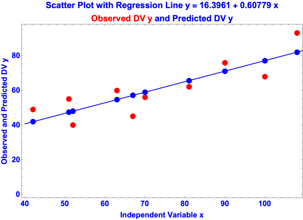
- The objective is to find an equation of the form y = a + bx that most accurately predicts the y’s from the x’s. That is, to find values for a and b that, given the observed x’s, predict y’s as close to the observed y’s as possible. That’s what the Least Squares Algorithm does. In this case the LSA determined that:
- a = 16.3961
- b = 0.60779
- So the regression equation is:
- y = 16.3961 + 0.60779 x

Example: Hubble’s Law
- Astronomers in the early 1900s observed distant galaxies moving directly away from us. In the late 1920s Edwin Hubble realized that the more distant a galaxy was, the faster it was receding.
- Here’s a graph of 735 faraway galaxies, with distances in megaparsecs.
- A megaparsec is 3.26 million lightyears
- The further away a galaxy is, the faster it recedes (in kilometers per second).
- Indeed, the correlation coefficient between distance and velocity is 0.818565, the scale going from -1 to 1.

- In 1929 Hubble set forth Hubble’s Law
- v = H0 x D, where
- D is distance from the Milky Way in megaparsecs
- v is the recessional velocity in kilometers per second
- H0 is Hubble’s Constant, somewhere between 67 and 73.
- v = H0 x D, where
- We’ll use simple linear regression to estimate Hubble’s Law.
- The data are the distances and velocities of 735 galaxies. For example:
- Thus the first galaxy on the list is 6.30377 megaparsecs from Earth, speeding away at 255.999 kilometers per second.


- The Least Squares Algorithm yields the regression equation: v = 59 d + 284, plotted in the chart as the straight line.
- v is the dependent variable, in kilometers per second
- d is the independent variable, in megaparsecs.
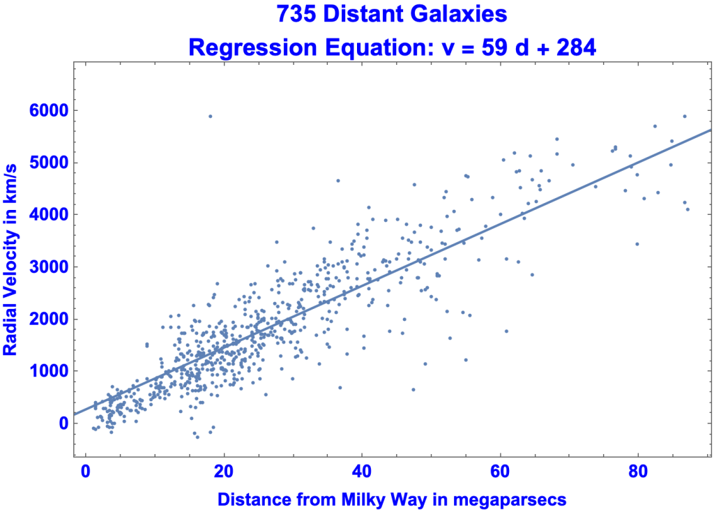
- The coefficient of d, 59, is less than Hubble’s Constant but in the ballpark
Multiple Linear Regression
Definition
- Simple Linear Regression yields an equation of the form y = a + bx that predicts values of the dependent variable y from the single independent variable x
- Multiple Linear Regression yields an equation whose form is y = b0 + b1 x1 + b2 x2 + … + bn xn, where
- y is the dependent variable
- x1 through xn are the independent variables
- b0 through bn are place-holder for real numbers
Example of Medications
- You take two medications to lower your blood pressure. To determine which is more effective you keep a daily log, with dosages and blood pressure.
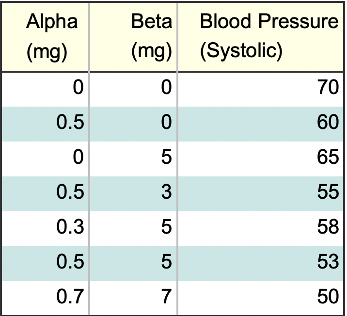
- The dosage for Drug Alpha is from 0.1 to 1 mg.
- The dosage for Beta is from 1 mg to 10 mg.
- The data in 3D:

- The medications are on the horizontal axes and blood pressure is on the vertical axis.
- The regression equation is:

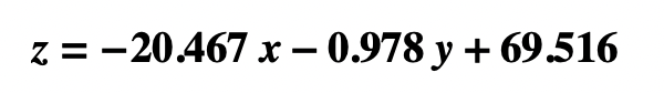
- where
- z is blood pressure
- x is the dosage of Drug Alpha
- y is the dosage of Drug Beta
- where
- So, for example, if Alpha = 0.5 mg and Beta = 3 mg (the fourth row on the data spreadsheet), the regression equation predicts:
- Which is pretty close to the observed value of 55.

Non-Linear Regression
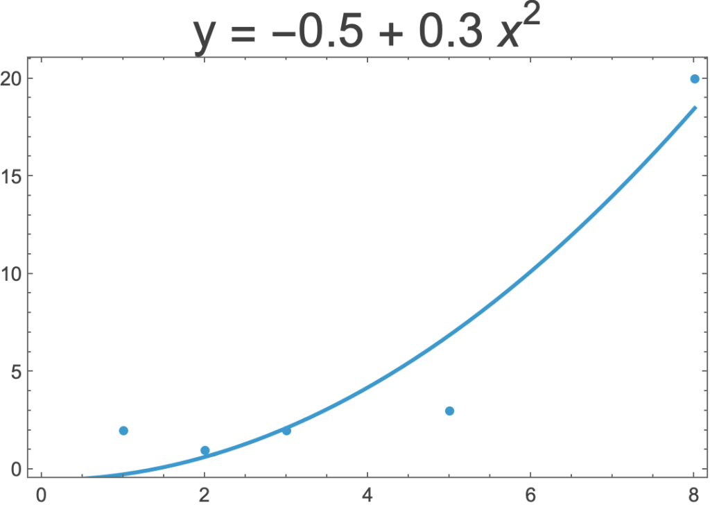
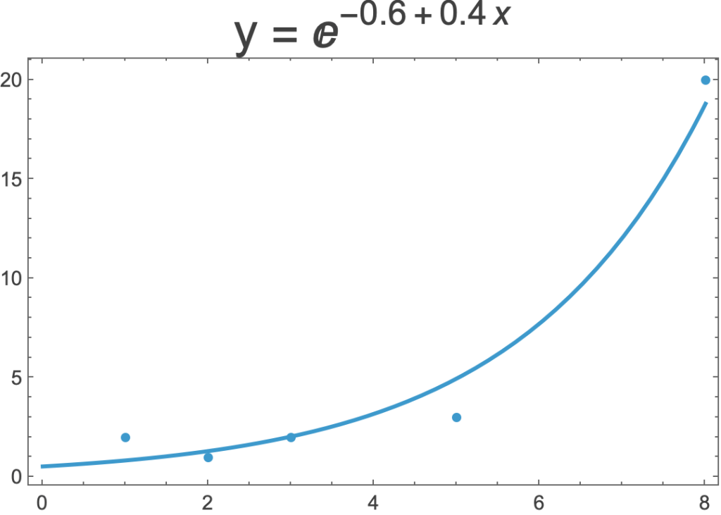
- Sometimes a straight line is not the best way to model a dataset.
- Here are three regressions of the same five data points.
- On the left is a linear regression.
- In the middle is non-linear regression that uses x2 rather x.
- On the right is a non-linear regression that uses the exponential function.

Evaluating Regressions
- The objective of regression is to find the simplest equation that most accurately predicts a dependent variable (DV) from independent variables (IVs).
- Evaluating a regression thus means assessing (1) the accuracy of its predictions and (2) the simplicity of its regression equation
Accuracy of Predictions
- The accuracy of a regression is how close the predicted values of the DV are to the observed values.
- The Least Squares Algorithm defines closeness as the residual sum of squares:

- That is:
- For each pair of observed and predicted values of the DV
- subtract the predicted from the observed value, yielding its residual
- square the residual
- Add up all the squares.
- For each pair of observed and predicted values of the DV
- View Residual Metrics
Simplicity of the Regression Equation
- The Principle of Simplicity (Ockham’s Razor, the Law of Parsimony) is that the simpler theory is more likely to be true, other things being equal.
- The Principle of Simplicity applies to the regression equation in two ways.
- First, the form of the regression equation should be as simple as possible, other things being equal. The equation y = a + bx, for example, is simpler than y = log(a + bx2)
- The simplest regression equations are linear equations, e.g.
- y = a + bx
- y = a + bx1 + cx2
- y = a + bx1 + cx2 + dx3
- Second, the set of indy variables should be as simple as possible, other things being equal. To paraphrase Ockham’s Razor
- Do not multiply independent variables beyond necessity.
Tools for Evaluating Regressions
Statisticians have developed various kinds of tools for evaluating regressions.
Graphics
- Graphics are essential to evaluating regressions. Indeed, different datasets can have nearly the same statistics but look totally different graphically.
- View Anscombe’s Quartet
- One of the most useful charts for simple linear regression is a scatter plot of the data with regression line.
- But graphs have limitations. For example, graphing the data and equation for a regression with two IV’s requires three dimensions.
- View Regression Graphics
Correlation
- Variables are correlated to the extent that they vary together, in the same or opposite directions.
- Correlation coefficients are useful
- between an independent variable and the dependent variable
- among independent variables
- The Correlation Matrix for multiple regression displays all the correlation coefficients between variables, independent and dependent.
- View Correlation Matrix
- View Correlation
Prediction
- An hypothesis is supported or disproved by its predictions. A regression equation is an hypothesis. So a natural way of evaluating a regression is to assess its predictions for “out-of-sample” data.
- An interesting metric, the Prediction Sum of Squares (PRESS), evaluates a regression by seeing how well regressions on the sample data, minus one datapoint, predict the missing data item.
Residual Metrics
- A residual is the difference, at a given datapoint, between the values of the observed and predicted dependent variable. There are different ways of combing the residuals into a single statistic.
- View Residual Metrics
Sum-of-Squares Metrics
- The Least Squares Algorithm is a method finding the equation that, given the observed values of the dependent and independent variables, yields the lowest possible residual sum of squares.
- The residual sum of squares, along with other sums of squares, is thus a natural basis for statistics that evaluate regressions.
- View Principle of Sums of Squares
- View R-Squared
- View Adjusted R-Squared
- View ANOVA for Simple Regression
- View ANOVA for Multiple Regression
Standard Error Metrics
- The standard error of an estimate is how statisticians quantify the idea of average error, i.e. as the standard distribution of the estimate’s sampling distribution.
- Of interest in regression are the standard errors of the regression, the mean of the residuals, the coefficients of the independent variables, and the intercept.
- View Standard Errors of the Regression, the Mean, the Independent Variables, and the Intercept
Likelihood Metrics
- Regression likelihood metrics are based on the idea that the more likely the data given the regression equation, the better the regression.
- The likelihood metrics also factor in the number of independent variables.
- View Likelihood Metrics
Example: Estimating Life Expectancy
- The objective of the example is to find an equation that predicts life expectancy by country from other statistics about countries, in particular:
- GDP per person employed
- Infant Mortality Fraction
- A number from 0 to 1 representing infant mortality
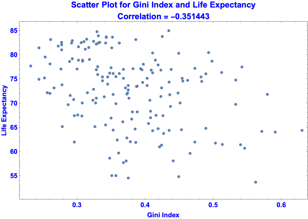
- Gini Index
- A number from 0 to 1 representing income inequality.
- I’ll evaluate the regressions using
- Graphs
- Correlations
- The following metrics
- Standard Error of the Regression
- t-Statistics for the standard errors of the coefficients
- R-Squared
- Adjusted R-Squared
- AICc
- The plan is to evaluate three sets of regressions:
- One Independent Variable
- Linear: GDP per person
- Linear: Infant Mortality Fraction
- Linear: Random Numbers
- NonLinear: GDP per person
- Two Independent Variables
- Linear: GDP per person & Infant Mortality Fraction
- NonLinear: GDP per person & Infant Mortality Fraction
- Linear: GDP per person, & Redundant Numbers
- Three Independent Variables
- Linear: GDP per person, Infant Mortality Fraction, Gini Index
- NonLinear: GDP per person, Infant Mortality Fraction, and Gini Index
- One Independent Variable
The Data
- The data is for 167 countries.
- Data items are:
- Name of country
- GDP per person employed
- Infant Mortality Fraction
- Gini Index
- Life Expectancy
- The Infant Mortality Fraction is the ratio of the number of children dying within one year of birth to the number dying within five years of birth.
- For our database of 167 countries:
- Mean IMF = 0.0281916
- Max IMF = 0.6477 South Sudan
- Min IMF = 0.0016 Slovenia
- US IMF = 0.0057
- The Gini Index is a measure of income inequality.
- As the Census Bureau puts it (Gini Index)
- “The Gini coefficient ranges from 0, indicating perfect equality (where everyone receives an equal share), to 1, perfect inequality (where only one recipient or group of recipients receives all the income).
- For our 167 countries
- Mean GI = 0.377154
- Max GI = 0.630 (South Africa}
- Min GI = 0.232 (Slovakia)
- US GI = 0.415
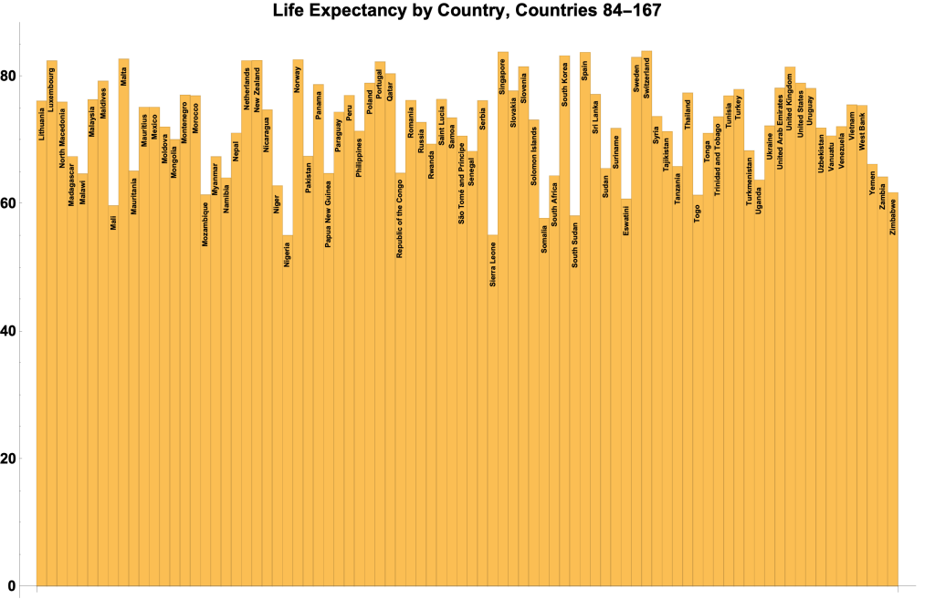
- Here are bar charts for life expectancy for the 167 countries:

Regression on One Independent Variable
Linear Regression on GDP
- A good place to start a regression is with a scatter plot and correlation coefficient for the variables:

- The data obviously shows a pattern. So we’ll run a regression GDP per Capita.
- Here’s a scatter plot with regression line and equation:

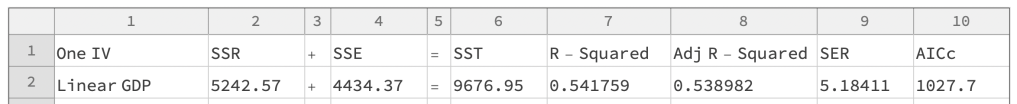
The regression stats:
- Regression Equation: y = 66.5212 + 0.000142379 $
- DataPoints = 167
- NbrofIVs = 1
- Sum of Squares Equation: 5242.57 + 4434.37 = 9676.95
- SSR + SSE = SST, where SSR, SSE, and SST are the sums of squares for
- predicted y’s,
- residuals,
- observed y’s
- SSR + SSE = SST, where SSR, SSE, and SST are the sums of squares for
- Standard Error of the Regression = 5.18411
- = √(SSE / (Datapoints – (NbrofIVs + 1)))
- R-Squared = 0.541759
- = SSR / SST
- Adjusted R-Squared = 0.538982
- AICc = 1027.7

- The average error is about four years per the mean absolute error (4.13141).
- So life expectancy is predicted to be so many years plus or minus four.
- The SER is a little more than this.
- R-Squared is 0.541759, meaning that the regression captures about 54% of the life expectancy scatter.
- The low P-values of the t-Statistics mean that the estimates for the coefficients are extremely accurate.
Linear Regression on IMF
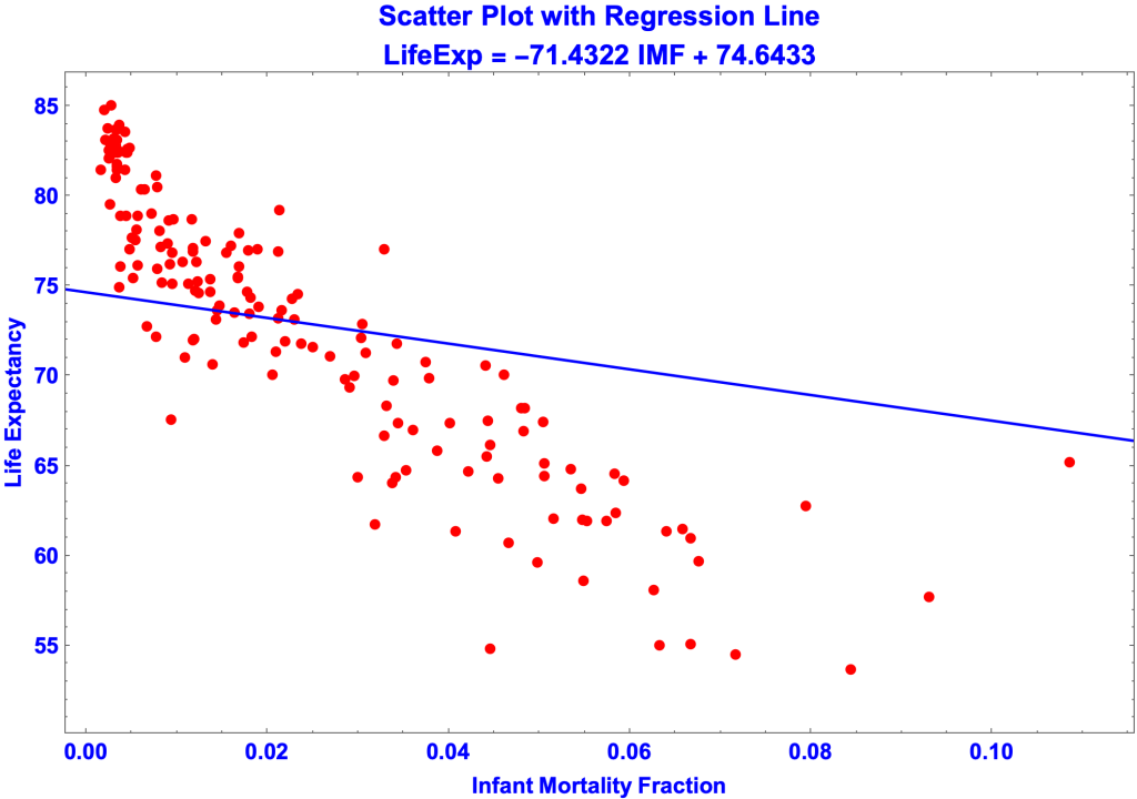
The regression stats are:
- Regression Equation: y = 74.6433 –71.4322 m
- DataPoints = 167
- NbrofIVs = 1
- Sum of Squares Equation: 2369.03 + 7307.92 = 9676.95
- SSR + SSE = SST, where SSR, SSE, and SST are the sums of squares for
- predicted y’s
- residuals
- observed y’s
- SSR + SSE = SST, where SSR, SSE, and SST are the sums of squares for
- Standard Error of the Regression = 6.6551
- = √(SSE / (Datapoints – (NbrofIVs + 1)))
- R-Squared = 0.244811
- = SSR / SST
- Adjusted R-Squared = 0.240234
- AICc = 1111.13

- The regression on IMF is not as good the regression on GDP
- SER is higher, 6.6551 versus 5.18411.
- R-Squared is lower, 0.244811 versus 0.541759
- AICc is higher, 1111.13 versus 1027.7
Linear Regression on Random Numbers

- Regression Equation: y = 64.5993 + 0.115757 x
- DataPoints = 167
- NbrofIVs = 1
- Sum of Squares Equation: 310.591 + 9366.35 = 9676.95
- SSR + SSE = SST, where SSR, SSE, and SST are the sums of squares for
- predicted y’s
- residuals
- observed y’s
- SSR + SSE = SST, where SSR, SSE, and SST are the sums of squares for
- Standard Error of the Regression = 7.53431
- = √(SSE / (Datapoints – (NbrofIVs + 1)))
- R-Squared = 0.032096
- = SSR / SST
- Adjusted R-Squared = 0.0262299
- AICc = 1152.57

- What stands out is the terribly low R-Square values, making this regression worthless.
Summary of Regression on One IV
Regression on Two Independent Variables
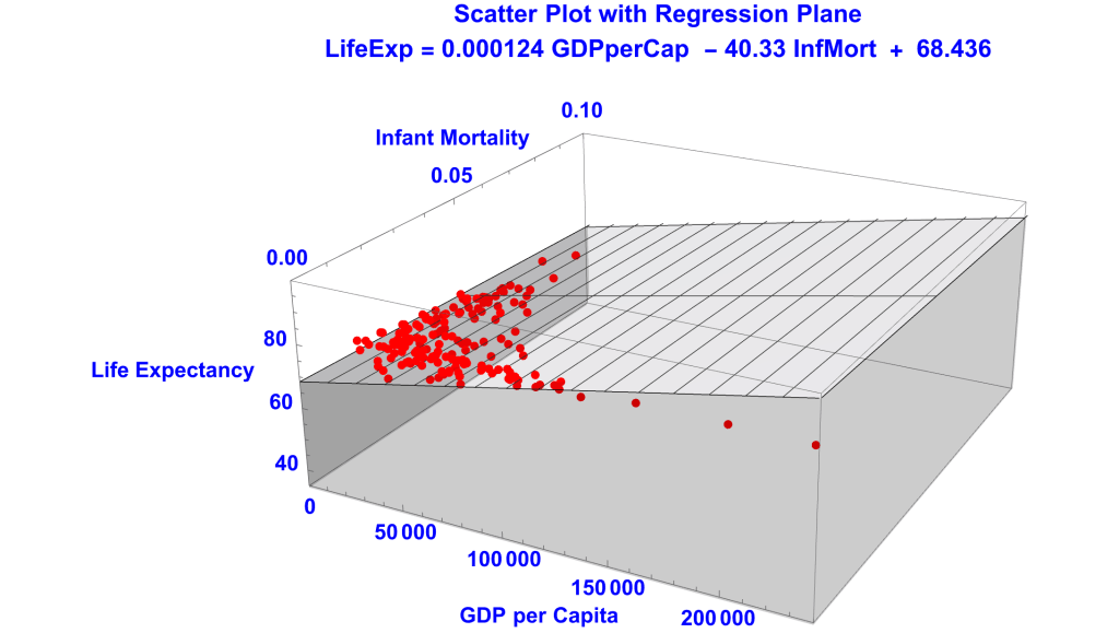
Linear Regression on GDP and IMF
IMF and LE are not as correlated as GDP and LE, 0.5 versus 7.4 in absolute values. That the former correlation is negative merely means that IMF and LE are correlated in opposite directions and is irrelevant to the accuracy of the regression.

The regression stats:
- Regression Equation; y = 68.4357 – 40.3304 m + 0.000124256 $
- DataPoints = 167
- NbrofIVs = 2
- Sum of Squares Equation: 5912.8 + 3764.14 = 9676.95
- SSR + SSE = SST, where SSR, SSE, and SST are the sums of squares for
- predicted y’s
- residuals
- observed y’s
- SSR + SSE = SST, where SSR, SSE, and SST are the sums of squares for
- Standard Error of the Regression = 4.79083
- = √(SSE / (Datapoints – (NbrofIVs + 1)))
- R-Squared = 0.61102
- = SSR / SST
- Adjusted R-Squared = 0.606276
- AICc = 1002.45

- So, the linear regression on GDP and IMF better fits the data than the simple linear regressions on GDP and IMF alone.
- The SER of 4.79083 is lower the SERS of 5.18411 and 6.6551.
- The R2 of 0.61102 is higher than the R2’s of 0.541759 and 0.244811.
- So progress has been made.
- But the linear regression on GDP and IMF does not score as well as the nonlinear regression on just GDP.
- The linear SER of 4.79083 is higher than the nonlinear SER of 4.31866
- The linear Adjusted-R2 of 0.606276 is lower than the nonlinear Adjusted-R2 of 0.68006.
- I switched to Adjusted-R2 since we’re comparing regressions with different numbers of IVs.
Linear Regression on GDP and Redundant GDP (1/3 times GDP)
- Regression Equation; y = 66.5212 + 0.000213569 r + 0.0000711895 $
- DataPoints = 167
- NbrofIVs = 2
- Sum of Squares Equation: 5242.57 + 4434.37 = 9676.95
- SSR + SSE = SST, where SSR, SSE, and SST are the sums of squares for
- predicted y’s
- residuals
- observed y’s
- SSR + SSE = SST, where SSR, SSE, and SST are the sums of squares for
- Standard Error of the Regression = 5.19989
- = √(SSE / (Datapoints – (NbrofIVs + 1)))
- R-Squared = 0.541759
- = SSR / SST
- Adjusted R-Squared = 0.536171
- AICc = 1029.82
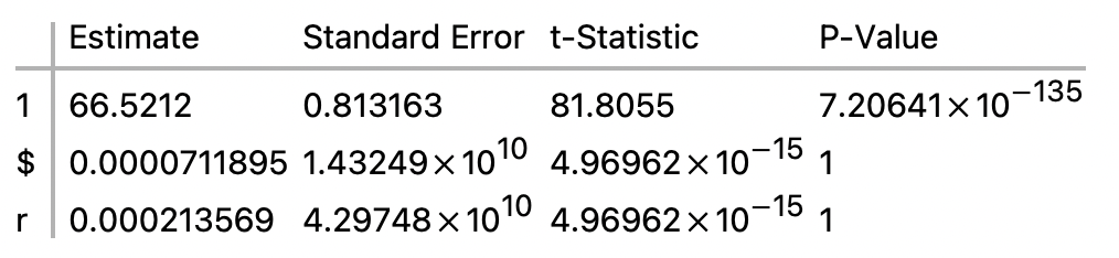
- This regression is on GDP and GDP/3, making the latter redundant.
- The sum of squares, and therefore R2 also, are the same as those for the regression on just GDP. But the Adjusted-R-Square is smaller, since it has an additional IV that contributes nothing to the regression.
- Redundant GDP = 0.536171
- GDP Alone = 0.538982
- And the SER is larger.
- Redundant GDP = 5.19989
- GDP Alone = 5.18411
Summary of Regression on Two IVs
Regression on Three Independent Variables
Linear Regression on GDP, IMF, and Gini
- Like IMF, the correlation of the Gini Index with Life Expectancy is negative. But the correlation is weaker.
- Regression Equation; y = 73.3606 – 12.435 g – 38.764 m + 0.00011775 $
- DataPoints = 167
- NbrofIVs = 3
- Sum of Squares Equation: 6057.69 + 3619.26 = 9676.95
- SSR + SSE = SST, where SSR, SSE, and SST are the sums of squares for
- predicted y’s
- residuals
- observed y’s
- SSR + SSE = SST, where SSR, SSE, and SST are the sums of squares for
- Standard Error of the Regression = 4.71212
- = √(SSE / (Datapoints – (NbrofIVs + 1)))
- R-Squared = 0.625992
- = SSR / SST
- Adjusted R-Squared = 0.619108
- AICc = 998.044

- This regression does better than the regression on just GDP and IMF.
- Take Adjusted R-Square, for example:
- Regression on GDP and IMF = 0.606276
- Regression on GDP, IMF, and Gini = 0.619108
Summary of Regression on Three IVs

Addendum
- Principle of Sums of Squares
- Standard Errors of the Regression, the Mean, the Independent Variables, and the Intercept
- More on Standard Error of the Regression
- R-Squared, the Coefficient of Determination
- Residual Metrics
- Regression Graphics
- Likelihood Metrics
- Least Squares Algorithm for Simple Linear Regression
- Quantifying Spread
- Epistemic justification for predicting unobserved values from observed values
- Regression to the Mean
- ANOVA for Regression
- ANOVA Table for Simple Linear Regression
- ANOVA Table for Multiple Linear Regression
- Anscombe’s Quartet
Principle of Sums of Squares
The Principle
- The Principle of the Sum of Squares is the basis for important metrics for evaluating linear regressions (and certain kinds of nonlinear regressions).
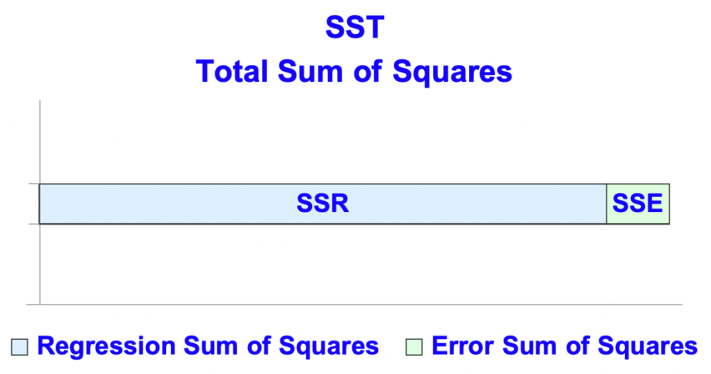
- The principle, using the common abbreviations:
- SSR + SSE = SST
- where
- SSR is the regression sum of squares
- SSE is the error (or residual) sum of squares
- SST is the total sum of squares.
- where
- SSR + SSE = SST
- From the values of SSR, SSE, and SST you can calculate:
- R-Squared
- Adjusted R-Squared
- Standard Error of the Regression
- Entries from the ANOVA table for regression such as Mean Squares, F-Statistic and its P-Value.
An Analogy
- Suppose you estimate the length of a small car that catches your eye
- The car is 10 feet long and you estimate 9 feet. So:

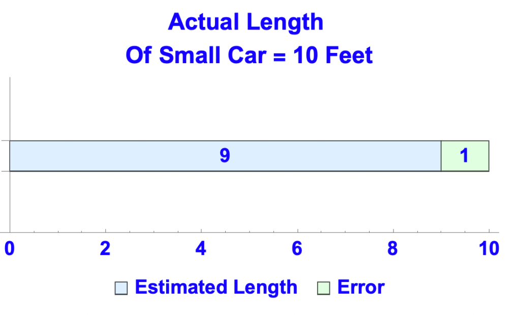
- SSR, SSE, and SST are the analogs of your estimate, the error, and the actual length of the car
- SSR represents the values of the dependent variable (DV) predicted by the regression
- SSE represents the difference between the observed and predicted values, what are called the residuals.
- SST represents the observed values of the DV
Definitions
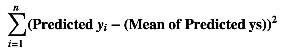
- SSR = the sum, for each predicted y, of (predicted y – mean of predicted ys)2
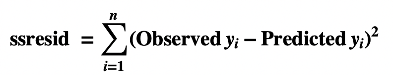
- SSE = the sum, for each y, of (observed y – predicted y)2
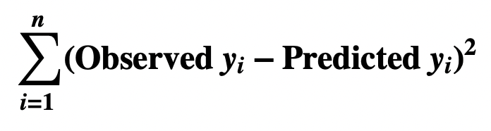
- A residual is an observed value of y minus its predicted value.
- So SSE = the sum of the squares of the residuals.
- The mean of the residuals is zero. Therefore an alternative definition of SSE is:
- the sum, for each predicted y, of (the residual at y – mean of the residuals)2
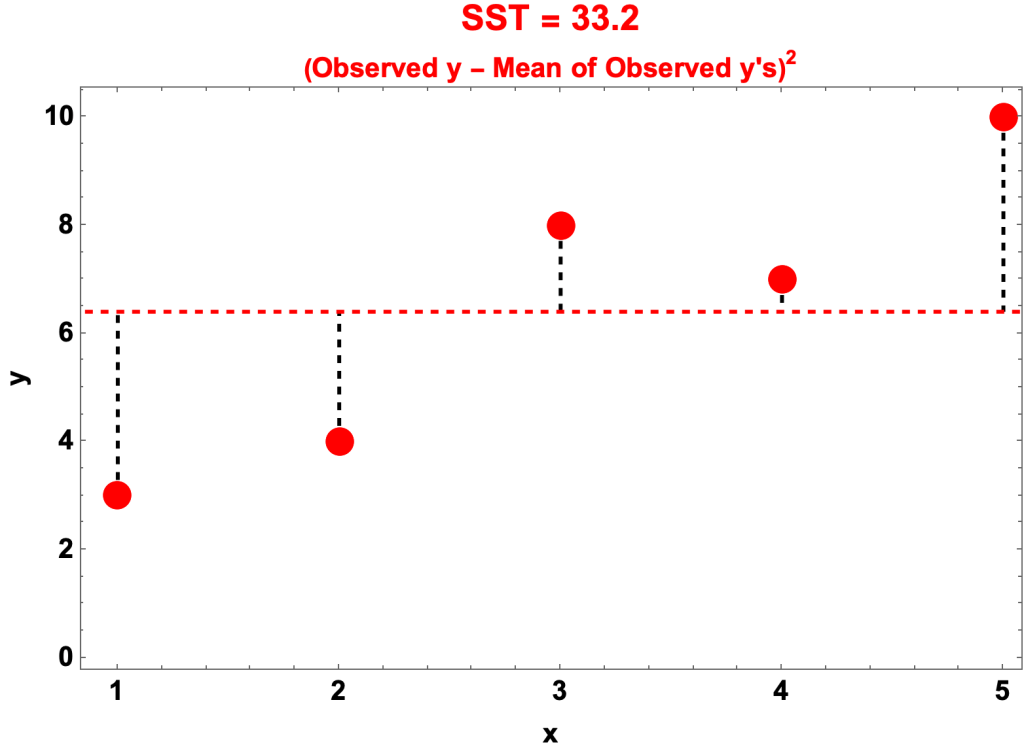
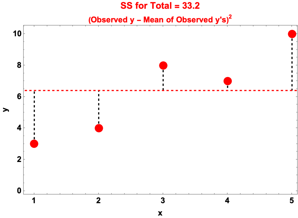
- SST = the sum, for each observed y, of (observed y – mean of observed ys)2
- Sum of Squares of x = the sum, for each x, of (x – mean of xs)2


Example
- The datapoints of the example are the pairs of x’s and y’s:
- data {x,y} = {1, 3}, {2, 4}, {3, 8}, {4, 7}, {5, 10}
- The x’s are the values of the independent variable (IV)
- The y’s are the observed values of the dependent variable (DV)
- The regression equation is y = 1.7 x + 1.3
- The predicted y’s, for x = 1 through 5, are:
- 3, 4.7, 6.4, 8.1, 9.8
- As we’ll see:
- SSR = 28.9
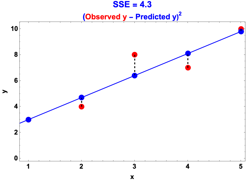
- SSE = 4.3
- SST = 33.2

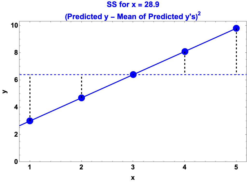
SSR, Regression Sum of Squares
- SSR = the sum of squares of the deviation of the predicted y’s from their mean
- For the example:

- In the graph
- The blue circles are the predicted y’s
- The solid, blue line is the regression line, y = 1.7x + 1.3
- The dashed, horizontal line is their mean, 6.4
- The dashed vertical lines are the distances from the predicted y’s to the mean
- SSR is the sum of the distances squared.

SSE, Residual Sum of Squares
- SSE = the sum of squares of the residuals
- In the example

- In the graph
- The solid, blue line is the regression line, y = 1.7x + 1.3
- The blue circles are the predicted y’s
- The red circles are the observed y’s
- The dashed vertical lines are the distances between the two
- SSE is the sum of the distances squared.
SST, Total Sum of Squares
- SSR = the sum of squares of the deviation of the observed y’s from their mean
- For the example: jwl

- In the graph
- The red circles are the observed y’s
- The dashed, horizontal line is the mean, 6.4
- The dashed vertical lines are the distances from the observed y’s to the mean
- SST is the sum of the distances squared.
Observations
- Variance of predicted y’s + variance of residuals = variance of observed y’s
- Mean of predicted y’s = mean of observed y’s
- Mean of residuals = 0

Statistics derived from SSR, SSE, SST
- R-Squared
- R-Squared = SSR/SST = 1 – (SSE/SST)
- View R-Squared
- Adjusted R-Squared
- Adjusted R-Squared adjusts R-Squared for number of data points and parameters
- View Adjusted R-Squared
- Standard Error of the Regression
- Standard Error of the Regression =

- where
- n = the number of datapoints
- k = the number of IVs
- View Standard Error of the Regression
- Standard Error of the Regression =
- Entries from the ANOVA table from regression
NonLinear Regression
- R-Squared presupposes the Principle of Sums of Squares. But, with some exceptions, the principle is false for nonlinear regressions, i.e. SSR + SSE ≠ SST. R-Squared makes no sense for such regressions.
- View R-Squared
Standard Errors of the Regression, the Mean, the Independent Variables, and the Intercept
Standard Error
- The standard error of an estimate is how statisticians quantify the idea of average error, i.e. as the standard distribution of the estimate’s sampling distribution.
- Consider a population statistic, perhaps average income or the percentage of people who are colorblind.
- Now take an n-size random sample and compute the statistic for the sample. It will undoubtedly differ from the population statistic. Now take a second n-size sample and compute its statistic. Then another and another until you’ve computed the statistic for hundreds of samples. The standard error of the statistic is the standard deviation of the all the sample statistics, known collectively as the sampling distribution of the statistic.
- There are formulas for estimating the standard error of various statistics from population parameters. The most well known is the formula for the mean of a population quantity: σ/√n, where
- σ is the standard deviation of the quantity in the population
- n is the size of the sample.
- Of interest in regression are the standard errors of the regression, the mean of the residuals, the coefficients of the independent variables, and the intercept.
Data for Examples
- datapoints = {{51, 55}, {100, 68}, {63, 60}, {52, 40}, {67, 45}, {42, 49}, {81, 62}, {70, 56}, {108, 93}, {90, 76}}
- xs = {51, 100, 63,52, 67, 42, 81, 70, 108, 90}
- ys = {55, 68, 60, 40, 45, 49, 62, 56, 93, 76}
- n = number of datapoints = 10
- k = number of independent variables = 1
- Regression Equation: y = 16.3961 + 0.607789 x
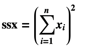
Two Sums of Squares and One Square of Sums
- Residual Sum of Squares
- Sum of Squares for x
- Square of Sum of the xs
- View Sums of Squares


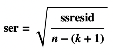
Standard Error of the Regression
- The Standard Error of the Regression, also called the Standard Error of the Estimate, is the standard deviation of the residuals:

- Observation
- The Standard Error of the Regression differs only slightly from the standard standard deviation:

Standard Error of the Mean
- The Standard Error of the Mean of the Residuals is computed using the standard formula for the standard error of the mean: σ/√n, where
- σ is the standard deviation of the population residuals, assumed to be the Standard Error of the Regression.
- n is the number of datapoints


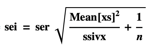
Standard Error of Independent Variable x


- Jonathan Gillard derives the formula in Chapter 7 of his First Course in Statistical Inference.
- Standard Error of independent variables can also be estimated using Monte Carlo simulation.
Standard Error of the Intercept

- Jonathan Gillard derives the formula in Chapter 7 of his First Course in Statistical Inference.
- Standard Error of intercepts can also be estimated using Monte Carlo simulation.
Parameter Table
- The regression equation for the example is:
- y = 16.3961 + 0.607789 x
- This is its Parameter Table:
- We’ve just calculated the standard errors.
- Now we’ll calculate the t-Statistics and the P-Values.
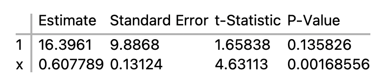
t-Statistic
- The standard error of an estimate only makes sense relative to the estimate. The t-Statistic in the parameter table is the ratio of the estimate to its standard error.
- tstat1 =16.39601 / 9.8868 = 1.65838
- tstatx = 0.607789 / 0.13124 = 4.63113
P-Value of a t-Statistic
- The significance of a t-Statistic can be understood in terms of probability, what’s called the P-value.
- The p-value of a t-Statistic is the probability of getting the same or a better t-Statistic by chance.
- A t-Statistic with a p-value is one in a million is excellent. A p-value of 1/2 is lousy.
- The formal definition:
- The p-value of a t-statistic T is the probability of getting a t-Statistic equal to or larger than |T| or equal to or smaller than –|T|, where the probability is determined by the Student’s t-distribution with n – (k + 1) degrees of freedom, n being the number of datapoints and k the number of independent variables.
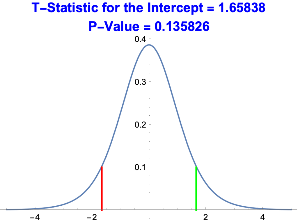
- Below is a plot of p-values against t-Statistics for the estimate of the intercept, 16.3961.
- The green line represents the t-Statistic, 1.65838.
- The red line represents –1.65838
- A better t-Statistic is one that’s greater than 1.65838 or less than –1.65838, i.e. to the right of the green line or to the left of the red line.
- The probability of that happening by chance is 0.135826, the area under the curve to the right of the green line and to the left of the red line. This is about one chance in ten. A poor p-value.
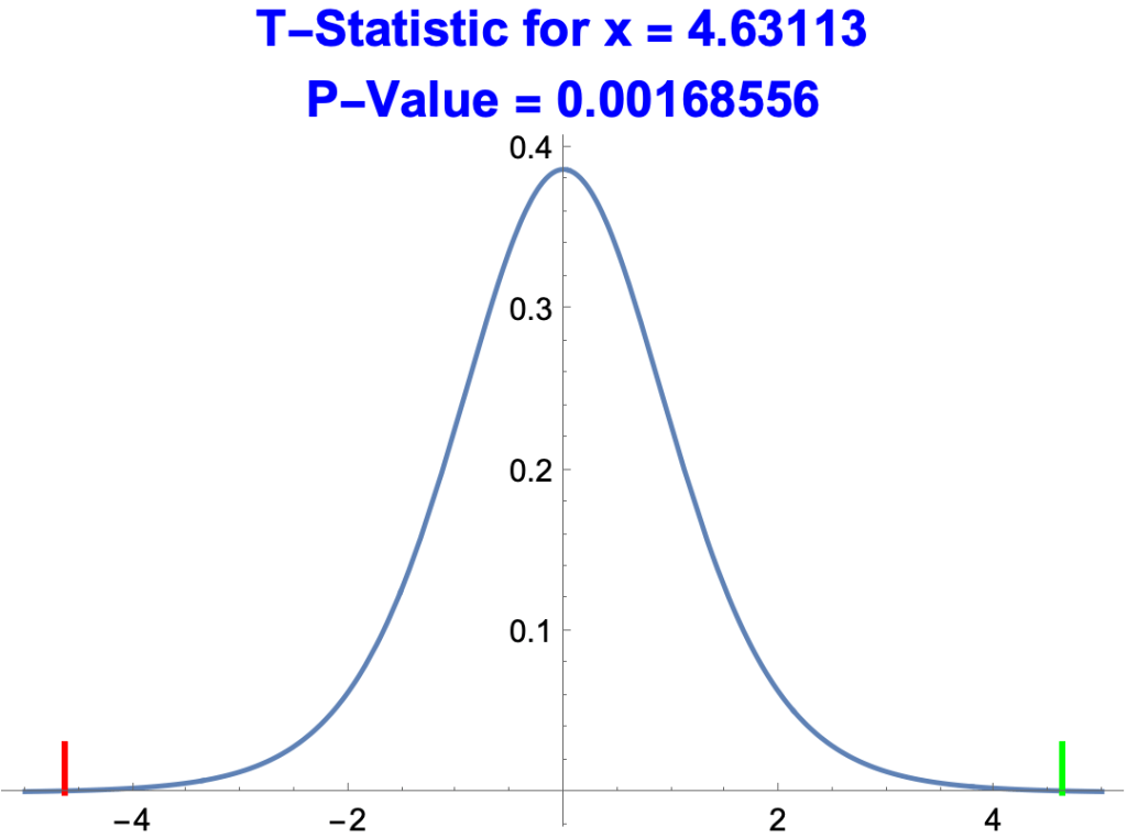
- Below is a plot of p-values against t-Statistics for the estimate of x, 0.607789.
- The green line represents the t-Statistic, 4.63113
- The red line represents –4.63113
- The probability of getter t-Statistic greater than 4.63113 or less than –4.63113 by chance is very low, 0.00168556, about 1 or 2 out of a thousand.
- The estimate for x is thus much better than the estimate for the intercept.
More on Standard Error of the Regression
- The Standard Error of the Regression, also called the Standard Error of the Estimate, is the standard deviation of the residuals, i.e. the square root of the residual sum of squares divided by n-(k+1):
- where
- n is the number of data points
- k is the number of IVs

The standard error of the regression can be regarded as a slightly exaggerated average error.
- Suppose a guy claims to be able to identify people’s ages. He makes ten guesses:
- {Real Age, Guess} = {{70, 73}, {35, 31},{46, 53},{48, 47},{28, 30},{22, 19},{66,59},{44,42},{82,76},{21,21}}
- How did he do?
- His ten guesses were off by:
- {3, 4, 7, 1, 2, 3, 7, 2, 6, 0}
- Which averages to 3.5.
- So his average error was 3.5 years, called the Mean Absolute Error (MAE) of his guesses.
- MAE’s are a perfectly good measure of estimates.
- MAE = Mean( | actual y – estimated y | )
- However, calculus has difficulty doing calculations with MAEs and absolute values in general.
- So statisticians use squares rather than absolute values.
- In this case they use the Root Mean Square (RMS) rather than the Mean Absolute Error (MAE)
- RMS = Sqrt( (actual y – estimated y)2 )
- RMS = √ Mean(9, 16, 49, 1, 4, 9, 49, 4, 36, 0) = 4.20714
- The Standard Error of the Regression is like the root mean square except that, in calculating the mean, you divide by n – (k +1) rather than just by n.
- The bottom line is that the standard error of the regression is like a slightly exaggerated average error.
R-Squared, the Coefficient of Determination
R-Squared
- R2, also known as the Coefficient of Determination, is a measure of how much of the scatter of an observed dependent variable is predicted (or explained) by the regression equation and the independent variables. Running from 0 to 1, R2 is conveniently thought of as a percent.
- R2 = SSR / SST
- where
- SSR = the regression sum of squares
- SST = the total sum of squares
- where
- R2 presupposes Principle of Sum of Squares. It follows that
- R2 = 1 – (SSE / SST)
- where
- SSE = the residual sum of squares
- where
- View Principle of Sums of Squares
- R2 = 1 – (SSE / SST)
- Example:
- The datapoints of the example are the pairs of x’s and y’s:
- data {x,y} = {1, 3}, {2, 4}, {3, 8}, {4, 7}, {5, 10}
- The x’s are the values of the independent variable (IV)
- The y’s are the observed values of the dependent variable (DV)
- The regression equation is y = 1.7 x + 1.3
- The predicted y’s, for x = 1 through 5, are:
- 3, 4.7, 6.4, 8.1, 9.8
- SSR = 28.9
- SSE = 4.3
- SST = 33.2
- The datapoints of the example are the pairs of x’s and y’s:
- So R2 = 28.9/33.2 = 0.870482
- For Simple Linear Regressions, the square root of R2 = the correlation coefficient of the x’s and observed y’s.
- Square root of 0.870482 = 0.932996
- Correlation of {1, 2, 3, 4, 5} and {3, 4, 8, 7, 10} = 0.932996
- For NonLinear Regressions, there’s no guarantee that SSR + SSE = SST, in which case R-Squared is invalid.
- For example, in the nonlinear regression for data {x, y} = {1, 3}, {2, 4}, {3, 8}, {4, 7}, {5, 10} where the regression equation is: y = log(146 x2 – 127):
- SSR = 9.2
- SSE = 17.38
- SST = 33.2
- But SSR + SSE = 26.6
- Some software packages do not compute R2. Others compute excessively high values. The bottom line is: don’t trust R2 for nonlinear regressions.

Adjusted R-Squared
- Adjusted R-Squared adjusts R-Squared for the number of datapoints and independent variables.
- Adjusted R-Squared =

- Where
- n = number of datapoints
- k = number of independent variables.
- Where
- Adjusted R-Squared is like R-Squared except that it factors in simplicity as well as accuracy.
- Here’s an example.
- Here are the results of a regression on two IVs: b and h
- Regression Equation = 111.276 + 2.06065 b – 2.72993 h
- Sum of Squares Equation: 5572.74 + 13321.8 = 18894.6
- (SSR + SSE = SST)
- R-Squared = 0.294939
- SSR / SST
- Adjusted R-Squared = 0.25465
- 1 – ( (DataPoints – 1)(1 – R-Squared) / (DataPoints – NbrofIVs – 1) )
- Here’s the same regression except with an additional, weak IV: w
- Regression Equation = 111.354 + 2.06037 b – 2.73193 h + 0.000559937 w
- Sum of Squares Equation: 5572.74 + 13321.8 = 18894.6
- (SSR + SSE = SST)
- R-Squared = 0.294939
- SSR / SST
- Adjusted R-Squared = 0.232728
- 1 – ( (DataPoints – 1)(1 – R-Squared) / (DataPoints – NbrofIVs – 1) )
- The sums of squares are the same (5572.74, 13321.8, 18894.6) and so therefore is R-Squared (0.294939). But Adjusted R-Squared went from 0.25465 to 0.232728, because of the additional IV.
- 1 – ( (38 – 1) (1 – 0.294939) / (38 – 2 – 1) ) = 0.25465
- 1 – ( (38 – 1) (1 – 0.294939) / (38 – 3 – 1) ) = 0.232728
Residual Metrics
Statistics used in the examples:
- data{x,y} = {{51,55},{100,68},{63,60},{52,40},{67,45},{42,49},{81,62},{70,56},{108,93},{90,76}}
- Regression Equation: y = 16.396 + 0.608 x
- Predicted ys = {47.3933, 77.175, 54.6868, 48.0011, 57.1179, 41.9232, 65.627, 58.9413, 82.0373, 71.0971}
- Residuals = {7.60668, -9.17497, 5.31322, -8.00111, -12.1179, 7.07678, -3.62698, -2.94131, 10.9627, 4.90292}
- n = the number of datapoints = 10
- k = the number of indy variables = 1
Absolute Values
- SAE: Sum of Absolute Errors

- MAE: Mean Absolute Error

Squares
- SSE: Sum of Squared Errors

- MSE: Mean Squared Error

- RMSE: Root Mean Square Error

- s: Standard Error of Regression

Regression Graphics
Scatter Plot with Regression Line
3D Scatter Plot with Regression Plane

Residual Plot

Normal Residual Plot

Correlation Matrix

Likelihood Metrics
The Idea
- A hypothesis is more likely if it better predicts the data than competing hypotheses, other things being equal.
- Regression Likelihood Metrics are based on the idea that the more likely the data given the regression, the better the regression.
- Specifically, the likelihood of the data given the regression is
- the maximum likelihood of the residuals given a normal distribution(μ,σ) where:
- the mean μ = 0 (the mean of the residuals).
- the standard deviation σ = the standard error the regression (which maximizes the likelihood)
- the maximum likelihood of the residuals given a normal distribution(μ,σ) where:
- Likelihoods are so small that statisticians instead use their logs and speak of the loglikelihood of the residuals, e.g talking about loglikelihood -34.7538 rather than the likelihood 8.06537*10-16
- We’ll look at three likelihood metrics : AIC, AICc, and BIC
- They all work the same way
- The smaller the metric, the better the regression
- Each has two components
- Maximum Likelihood Component
- – 2 maximum loglikelihood
- The higher the max likelihood the lower the metric
- Likelihood of 8-5 yields a -2 max loglikelihood of 20.7944
- Likelihood of 8-20 yields a -2 max loglikelihood of 83.1777
- Complexity Penalty
- The more complex the regression, the higher the metric
- Maximum Likelihood Component
Data for Examples
- datapoints{x,y} = {{51, 55}, {100, 68}, {63, 60}, {52, 40}, {67, 45}, {42, 49}, {81, 62}, {70, 56}, {108, 93}, {90, 76}}
- Regression Equation: y = 16.3961 + 0.607789 x
- Residuals = {7.60668, -9.17497, 5.31322, -8.00111, -12.1179, 7.07678, -3.62698, -2.94131, 10.9627, 4.90292}
- Standard Error of the Regression = 8.64032
AIC, the Akaike Information Criterion
- AIC = – 2 max loglikelihood + 2 k, where k = 1 + the number of estimated parameters
- Example
- AIC = -2 (max log likelihood of residuals given the normal distribution(μ,σ)) + 2 k
- -2 (max log likelihood of residuals given the normal distribution(0,8.64032)) + 2 k
- (- 2 )(-34.753781) + (2 * 3)
- 69.5076 + 6
- AIC = 75.5076
- So AIC adds a penalty of 6 for the number of individual variables
- AIC = -2 (max log likelihood of residuals given the normal distribution(μ,σ)) + 2 k
AICc, the Corrected Akaike Information Criterion
- AICc = AIC + (2 k (k + 1))/(n – k – 1), where k = 1 + the number of estimated parameters
- Example
- AICc = AIC + (2 k (k + 1))/(n – k – 1)
- 75.5076 + (6 * 4) / (10-3-1)
- 75.5076 + 4
- AICc = 79.5076
- AICc = AIC + (2 k (k + 1))/(n – k – 1)
- (2 k (k + 1))/(n – k – 1) imposes a penalty for a small number datapoints, for example, where k = 3, the penalty is:
- 24 for n = 5 datapoints
- 4 for n = 10 datapoints
- 1.5 for n = 20 datapoints
BIC, Bayesian Information Criterion
- BIC = -2 (max log likelihood of residuals given the normal distribution(μ,σ)) + k Log[n], where k = 1 + the number of estimated parameters
- Example
- BIC = -2 (max log likelihood of residuals given the normal distribution(μ,σ)) + k Log[n]
- -2 (max log likelihood of residuals given the normal distribution(0,8.64032)) + 3 Log[10]
- (-2 )(-34.753781) + (3 * 2.30259)
- 69.5076 + 6.90777
- BIC = 76.4153
- BIC = -2 (max log likelihood of residuals given the normal distribution(μ,σ)) + k Log[n]
- BIC is like AIC except that its complexity penalty increases (gradually) with the number of datapoints:
- k Log[10] = 2.3 k
- k Log[100] = 4.6 k
- k Log[1000] = 6.9 k
Least Squares Algorithm for Simple Linear Regression
Overview
- In simple linear regression the regression equation has the form of a straight line:
- y = a + b x
- The objective is find a and b that, given the observed x’s, predict y’s as close to the observed y’s as possible.
- But how do you calculate “as close as possible?”
- One idea would be to select a and b to minimize the sum of absolute residuals.
- A residual is the difference between an observed y and a predicted y.
- The sum of absolute residuals = the sum of the absolute value of (observed y – predicted y) for all the observed y’s.
- Suppose that
- the observed y’s are 55, 68, 60, 40, 45, 49, 62, 56, 93, 76
- the predicted y’s are 47, 77, 55, 48, 57, 42, 66, 59, 82, 71
- The sum of the absolute residuals would then be:
- For mathematical reasons, statisticians instead try to minimize the sum of squares of residuals,
- The residual sum of squares is the sum of the (observed y – predicted y)2 for all the y’s. So squares replace absolute values.
- Suppose again that
- the observed y’s are 55, 68, 60, 40, 45, 49, 62, 56, 93, 76
- the predicted y’s are 47.3933, 77.175, 54.6868, 48.0011, 57.1179, 41.9232, 65.627, 58.9413, 82.0373, 71.0971
- The residual sum of squares is then:


- The Least Squares Algorithm is a method for calculating a and b such that, given the observed x’s and y’s, the equation y = a + b x yields the lowest possible residual sum of squares.
- For observed and predicted y’s
- Observed: 55, 68, 60, 40, 45, 49, 62, 56, 93, 76
- Predicted: 47.3933, 77.175, 54.6868, 48.0011, 57.1179, 41.9232, 65.627, 58.9413, 82.0373, 71.0971
- the Least Squares Algorithm generates
- a = 16.3961
- b = 0.607789
- So the regression equation is:
- y = 16.3961 + 0.607789 x
- And the least residual sum of squares is 597.241
- So, for the given x’s and y’s, no a and b yield a lower residual sum of squares.
The Math
- Given particular x’s and y’s we want to find an a and b such that y = a + b x yields the smallest residual sum of squares:
- Graphically, we want to find the lowest point of the curved surface representing RSS as a function of a and b


- That is, we want to find the point where
- The rate of change of the slope of the surface with respect to a = 0
- The rate of change of the slope of the surface with respect to b = 0
- Which are differential equations:
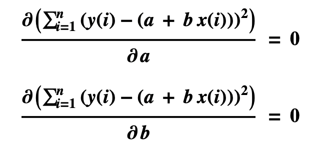
- Taking the derivatives of the left sides yields

- These equations can be solved for particular values of x and y, e.g.
- x[i] = 51, 100, 63, 52, 67, 42, 81, 70, 108, 90, for i = 1 through 10
- y[i] = 55, 68, 60, 40, 45, 49, 62, 56, 93, 76, for i = 1 through 10

- Solving the equations simultaneously yields the coefficients a and b

- The regression equation is therefore:
- y = 16.3961 + 0.607789 x
Quantifying Spread
- Statisticians quantify spread in several inter-definable ways.
- Spread is also called dispersion or scatter.
- Take a collection numbers, e.g.
- {1, 6, 2, 7, 2, 8, 3, 8, 8, 5}
- A scatter plot shows the spread:

- The average (mean), 5, can be represented as a line:

- The spread (dispersion, scatter) of the datapoints is be represented as their aggregate distance from the mean.
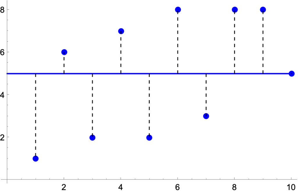
- It’s easy to calculate the combined length of the dashes.
- |1-5| + |6-5| + |2-5| + |7-5| + |2-5| + |8-5| + |3-5| + |8-5| + |8-5| + |5-5| = 24
- where |x| is the absolute value of x, i.e the positive version of x. So |1-5| = 4
- The average length is thus 24 / 10 = 2.4
- So if you laid out ten golf balls on a basketball court per the graph, using the mid-court line as the mean, and measuring distances in feet, then
- The total distance of the golf balls from the mid-court line would be 24 feet.
- The average distance would be 2.4 feet.
- |1-5| + |6-5| + |2-5| + |7-5| + |2-5| + |8-5| + |3-5| + |8-5| + |8-5| + |5-5| = 24
- But statisticians have found it’s more mathematically convenient to use squares rather than absolute values, e.g. (1-5)2 instead of |1-5 |.
- There are three inter-definable notions used to quantify spread:
- Sum of Squares
- The sum of (n – mean)2
- (1-5)2 + (6-5)2 + (2-5)2 + (7-5)2 + (2-5)2 + (8-5)2 + (3-5)2 + (8-5)2 + (8-5)2 + (5-5)2 = 70
- Variance
- The sum of (n – mean)2 divided by the number of datapoints minus one
- 70 / (10-1) = 7.8
- Standard Deviation
- The square root of the variance
- √7.8 = 2.79
- The square root of the variance
- Sum of Squares
- Any of these statistics can be calculated from any of the others if you know the number of datapoints, e.g.
- 2.792 x (10 – 1) = 70
Epistemic justification for predicting unobserved values from observed values
- The regression equation E is the simplest equation that most accurately predicts the observed values of a dependent variable from the observed values of a set of independent variables.
- Therefore, E is likely to accurately predict unobserved values of the dependent variable from unobserved values of the independent variables, other things being equal
Regression to the Mean
- Regression Toward the Mean is a statistical phenomenon where a quantity measured far above or below average is likely to be closer to the mean on a second measurement. Inferring a causal explanation for a lower measurement is the Regression Fallacy.
- The explanation of RTM is twofold:
- Measurements are a function of both the measured quantity and chance.
- The measured quantity is not evenly distributed.
Part 1 of the Explanation
- Measurements depend on both the measured quantity and chance. A student’s score on an exam, for example, depends both on what the student knows and luck.
- Suppose that five test takers have the same high level of knowledge, specifically knowledge at the 90 grade-level. The students thus score 90 on exams give or take, where “give or take” is a matter of chance.
- The probability distribution of test grades for a student with 90 grade-level knowledge:

- The test-takers, A, B, C, D, and E, score 99, 95, 89, 87, and 82 respectively.
- We would expect student A to do worse on a retest since by chance she scored far above her 90 grade-level knowledge. And we would expect student E’s score to improve on a second exam.
- In a computer simulation, 1,000 students with 90 grade-level knowledge take a test. They take a second test on the same material but with different questions The results are:
- Of those who scored at least 92 on the first exam, 81 percent did worse on the second exam.
- Of those who scored at most 85 on the first exam, 90.5 percent did better on the second exam.
Part 2 of the Explanation
- Suppose a student gets a 90 on a test and that’s all we know. In particular, we don’t know the student’s grade-level knowledge. Perhaps she’s a student with 97 grade-level knowledge, had a bad day, and will probably do better on a retest. Or maybe she’s a student with 83 grade-level knowledge, got lucky on the exam, and will probably do worse on the next test.
- It would seem equally likely that
- (a) the student’s knowledge is above the 90 grade-level and her test score was bad luck
- (b) the student’s knowledge is below the 90 grade-level and she lucked out on the exam.
- But (a) and (b) are not equally likely. Possibility (b) is more likely than (a) and therefore the student’s score on a retest is more likely to be lower than higher.
- Here’s why.
- Knowledge levels are typically normally distributed. Let’s assume that the average knowledge level of a class is 75 and the distribution is normal. That is:
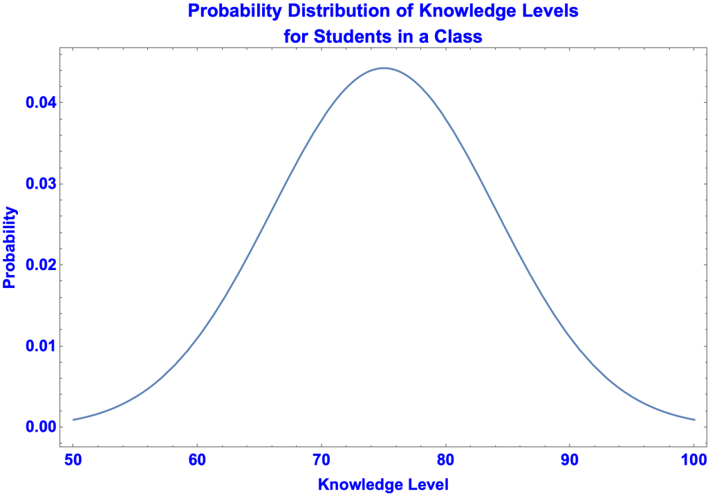
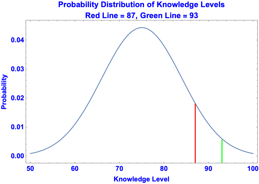
- Suppose a student scores 90 on an exam. Her knowledge level is more likely to be 89 than 91, more likely to be 88 than 92, more likely to be 87 than 93, and so on. The reason is that knowledge levels are normally distributed. Thus, for example, the probability of a randomly selected student having a 93 knowledge level (0.0079) is less than a student having an 87 knowledge level (0.0194). That is, the green line on the graph is shorter than the red line.
- For each knowledge level (let’s assume there are 100) we can compute:
- the probability of a student having that knowledge level
- the probability of a student with that knowledge level scoring higher than 90.
- Thus, the probability of a student having a certain knowledge level and scoring higher than 90 is the product of the two probabilities. For example, the probability of a student having an 87 knowledge level and scoring above 90 is 0.019 x 0.334= 0.00649.
- Combining the probabilities of scoring above and below 90 for all 100 knowledge levels yields:
- The probability of scoring higher than 90 = 0.1
- The probability of scoring lower than 90 = 0.9
- Thus, not knowing her knowledge level, but assuming knowledge levels are normally distributed, the student who scored 90 on the exam will, in all likelihood, do worse on a retest.
Regression Fallacy
- The regression fallacy is inferring that an instance of regression to the mean is due to something other than chance.
- Here’s an example in the words of Daniel Kahneman
- “I had the most satisfying Eureka experience of my career while attempting to teach flight instructors that praise is more effective than punishment for promoting skill-learning. When I had finished my enthusiastic speech, one of the most seasoned instructors in the audience raised his hand and made his own short speech, which began by conceding that positive reinforcement might be good for the birds, but went on to deny that it was optimal for flight cadets. He said, “On many occasions I have praised flight cadets for clean execution of some aerobatic maneuver, and in general when they try it again, they do worse. On the other hand, I have often screamed at cadets for bad execution, and in general they do better the next time. So please don’t tell us that reinforcement works and punishment does not, because the opposite is the case.” This was a joyous moment, in which I understood an important truth about the world: because we tend to reward others when they do well and punish them when they do badly, and because there is regression to the mean, it is part of the human condition that we are statistically punished for rewarding others and rewarded for punishing them. I immediately arranged a demonstration in which each participant tossed two coins at a target behind his back, without any feedback. We measured the distances from the target and could see that those who had done best the first time had mostly deteriorated on their second try, and vice versa. But I knew that this demonstration would not undo the effects of lifelong exposure to a perverse contingency.”
History
- britannica.com/topic/regression-to-the-mean
- “An early example of RTM may be found in the work of Sir Francis Galton on heritability of height. He observed that tall parents tended to have somewhat shorter children than would be expected given their parents’ extreme height. Seeking an empirical answer, Galton measured the height of 930 adult children and their parents and calculated the average height of the parents. He noted that when the average height of the parents was greater than the mean of the population, the children were shorter than their parents. Likewise, when the average height of the parents was shorter than the population mean, the children were taller than their parents. Galton called this phenomenon regression toward mediocrity; it is now called RTM. This is a statistical, not a genetic, phenomenon.”
ANOVA for Regression
Basic Idea
- ANOVA, the Analysis of Variance, is a method for determining whether a significant difference exists among the means of more than two groups of data.
- It is also used for evaluating regressions.
- ANOVA is most easily explained by analogy.
- Suppose you estimate the length of a small car that catches your eye.
- The car is 10 feet long and you estimate 9 feet.

- The same thing goes on in regression and ANOVA.
- In a regression
- Values of x and y are observed.
- A regression is run
- The regression equation predicts y’s from the x’s
- In an ANOVA analysis of regression
- A first number is calculated, SST, representing the observed y’s.
- A second number is calculated, SSR, representing the predicted y’s.
- A third number is calculated, SSE, representing the difference between the observed and predicted y’s
- Just as the predicted length of the car + error = the actual length of the car, SSR + SSE = SST
More on R-Squared
ANOVA Table for Simple Linear Regression
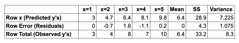
ANOVA Table
- We’ll use the example we’ve been using
- Data {x, y} = {1, 3}, {2, 4}, {3, 8}, {4, 7}, {5, 10}
- Regression Equation: y = 1.7 x + 1.3
- The ANOVA table for the regression:

Where are the Variances?
- You’d expect a table for the analysis of variances would at least have a column for variances. Actually the variances are easily calculated by dividing the SS column figures by DF for Total, i.e.
- Variance for Row x = 28.9 / 4 = 7.225
- Variance for Row Error = 4.3 /4 = 1.075
- Variance for Row Total = 33.2 / 4 = 8.3
Rows
- Row x represents the predicted y’s
- Row Error represents the residuals
- Row Total represents the observed y’s
SS Column
SS for x
- SS for x = the sum of squares of the deviation of the predicted y’s from their mean
- That is, the sum of squares of (predicted y – mean of predicted y’s) for each y.
- For the example
- In the graph
- The blue circles are the predicted y’s
- The solid, blue line is the regression line
- The dashed, horizontal line is the mean, 6.4
- The dashed vertical lines are the distances from the predicted y’s to the mean
- These distances are squared and summed.
SS for Error
- SS for Error = the sum of the squares of the deviation of the residuals from their mean
- That is, the sum of the squares of residual – mean of the residuals)
- The mean of the residuals is always zero.
- So SS for Error reduces to the sum of the squares of (observed y – predicted y) for each y
- For the example
- In the graph
- The green circles are the residuals
- The dashed, horizontal line is the mean, 0
- The dashed vertical lines are the distances from the residuals to the mean

- In this alternative graph
- The blue circles are the predicted y’s
- The red circles are the observed y’s
- The dashed vertical lines are the distances between the two

SS for Total
- SS for Total = the sum of squares of the deviation of the observed y’s from their mean
- That is, the sum of squares of (observed y – mean of observed y’s) for each y.
- For the example
- In the graph
- The red circles are the observed y’s
- The dashed, horizontal line is the mean, 6.4
- The dashed vertical lines are the distances from the observed y’s to the mean
SS Column Generalizations
- Variance of predicted y’s + variance of residuals = variance of observed y’s
- Sum of (predicted y’s – mean of predicted y’s)2 + sum of (residuals – mean of residuals)2 = sum of (observed y’s – mean of observed y’s)2
- Mean of predicted y’s = mean of observed y’s
- Mean of residuals = 0
DF and MS Columns
- The total degrees of freedom is the number of data points minus one = 5 – 1 = 4
- The df’s are then distributed as follows:
- One df to each independent variable
- So DF for x = 1
- The remaining df’s go to the Error line.
- So DF for Error = 3
- One df to each independent variable
- The mean squares are sums of squares divided by their degrees of freedom.
- 28.9 / 1 = 28.9
- 4.3 / 3 = 1.43333
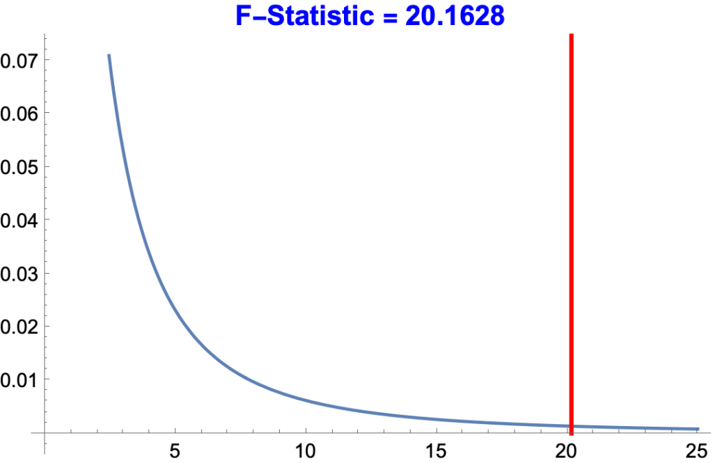
F-Statistic and P-Value Columns
- The F-statistic is the ratio of one MS to another.
- In the present case
- MS for x / MS for Error = 28.9 / 1.43333 = 20.1628
- The P-Value for a given F-Statistic is the probability of getting an F-Statistic as high or higher by chance.
- The probability of getting x ≥ 20.1628 for dfs 1 and 3 = 0.0206096, about 1 in 500.
- The higher the F-Statistic, the lower the p-value and the more accurate the predicted y’s.
- In the graph, the area under the curve to the right of the 20.1628 line = 0.0206096.
R2, the Coefficient of Determination
- R-Squared, the Coefficient of Determination, is the sum of the squares of (the predicted y’s – the mean of predicted y’s) divided by the sum of squares of (the observed y’s – the mean of the observed y’s).
- SS for x / SS for Total
- 28.9 / 33.2 = 0.870482
- SS for x / SS for Total
More on R-Squared
ANOVA Table for Multiple Linear Regression
A Study of IQ, Brain Size, Height and Weight
- The objective of a 1991 study of 38 college students by Willerman et al. was to see whether performance IQ could be predicted from brain size (based on MRI scans), height in inches, and weight in pounds.
The Data
- The data in the form {brain size, height, weight, PIQ} :
- {{81.69,64.5,118,124},{103.84,73.3,143,150},{96.54,68.8,172,128},{95.15,65.,147,134},{92.88,69.,146,110},{99.13,64.5,138,131},{85.43,66.,175,98},{90.49,66.3,134,84},{95.55,68.8,172,147},{83.39,64.5,118,124},{107.95,70.,151,128},{92.41,69.,155,124},{85.65,70.5,155,147},{87.89,66.,146,90},{86.54,68.,135,96},{85.22,68.5,127,120},{94.51,73.5,178,102},{80.8,66.3,136,84},{88.91,70.,180,86},{90.59,76.5,186,84},{79.06,62.,122,134},{95.5,68.,132,128},{83.18,63.,114,102},{93.55,72.,171,131},{79.86,68.,140,84},{106.25,77.,187,110},{79.35,63.,106,72},{86.67,66.5,159,124},{85.78,62.5,127,132},{94.96,67.,191,137},{99.79,75.5,192,110},{88.,69.,181,86},{83.43,66.5,143,81},{94.81,66.5,153,128},{94.94,70.5,144,124},{89.4,64.5,139,94},{93.,74.,148,74},{93.59,75.5,179,89}}
Regression Equation
- piq = 111.35 + 2.06 b – 2.73 h + 0.0005 w
Top-level ANOVA Table
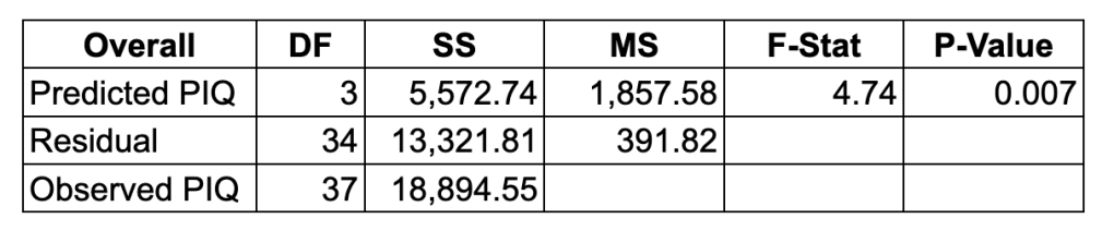
- SS for Predicted PIQ = the sum of (predicted piq of student x – mean of predicted piqs)2 , for every student x
- The DF = 3 since there are three independent variables
- SS for Residuals = sum (observed piq of student x – predicted piq of x)2 , for every student x
- SS for Observed PIQ = the sum of (observed piq of student x – mean of observed piqs)2 , for every student x
- SS for Predicted PIQ + SS for Residuals = SS for Observed PIQ
- 5,572.744 + 13,321.808 = 18,894.55
- R-Squared = 5,572.744 / 18,894.55 = 0.294939
ANOVA Table with Independent Variables
- We’ve calculated the sum of squares for the Predicted PIQ. The question now is: what part of that sum of squares is due to each independent variable? That is, we want to extend the top-level ANOVA table to brain size, height, and weight. Unfortunately there are two ways of doing this.
- Sequential Sum of Squares

- Partial (or Adjusted) Sum of Squares
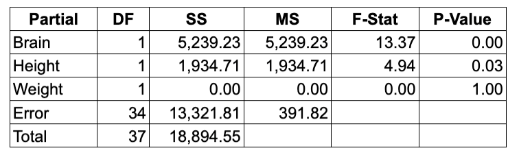
- The SS numbers for Brain, Height and Weight differ and therefore so do those for MS, F-Stat and P-Value.
- The rows for Error and Total are the same.
- There are curious things about both tables.
- First, the SS numbers of the Partial table don’t add up to 18,894.55
- 5,239.23 + 1,934.71 + 0 + 13,321.81 = 20,495.75
- Second, the SS numbers of the Sequential table change if you change the order of the independent variables:

- The weight, height, and brain SS numbers all different.
Calculation of Sequential Sum of Squares
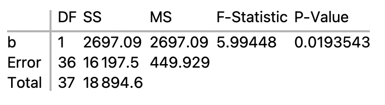
- We want to figure out where the SS numbers for brain, height, and weight come from in the sequential table:

- SS for b, 2697.02, comes from the simple linear regression for b.
- SS for h, 2875.65, comes from the multiple regression for b and h
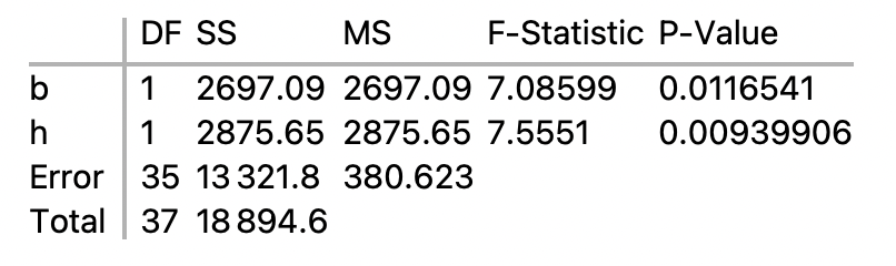
- In the multiple regression, SS for b is the same as in the SLR. SS for h is what remains from the total SS after all other SS’s are deducted, i.e.
- SS for h = SS for Total – SS for Error – SS for b
- 2,875.65 = 18,894.55 – 13,321.808 – 2,697.09
- SS for h = SS for Total – SS for Error – SS for b
- Finally, SS for w is what remains of the total SS in the ANOVA table for b, h, and w after all other SS’s are deducted, i.e.
- SS for w = SS for Total – SS for Error – SS for b – SS for h
- 0.00316329 = 18894.5526315789 – 13321.80819616275 – 2697.0939160885227 – 2875.6473560391623
Calculation of Partial Sum of Squares
- The table for the partial sum of squares is:
- A partial sum of squares in a multiple regression is what remains after the sum of squares for the other independent variables have been deducted from the sum of squares from the predicted dependent variable.
- To compute the partial sum of squares for brain size, run a multiple regression for the sequential sum of squares with brain size last:
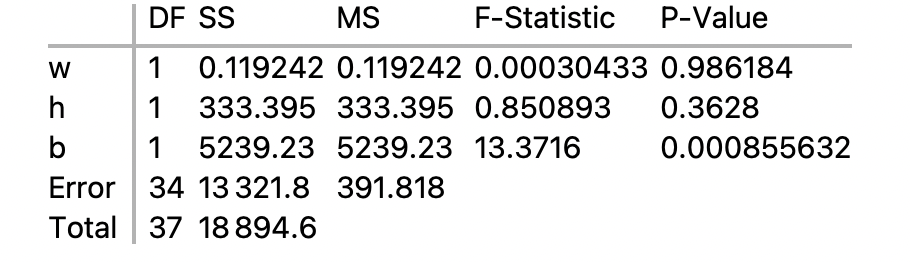
- The SS for b, 5239.23, is the partial sum of squares for brain size.
- This tells us that brain size substantially increased the sum of squares for the predicted piq, even after the variable for weight and height had already had their shot,
- To compute the partial sum of squares for height, run a multiple regression for the sequential sum of squares with height last:

- The SS for h, 1934.71, is the partial sum of squares for height.
- And the SS for weight, 0, derives from a multiple regression for the sequential sum of squares with weight last:

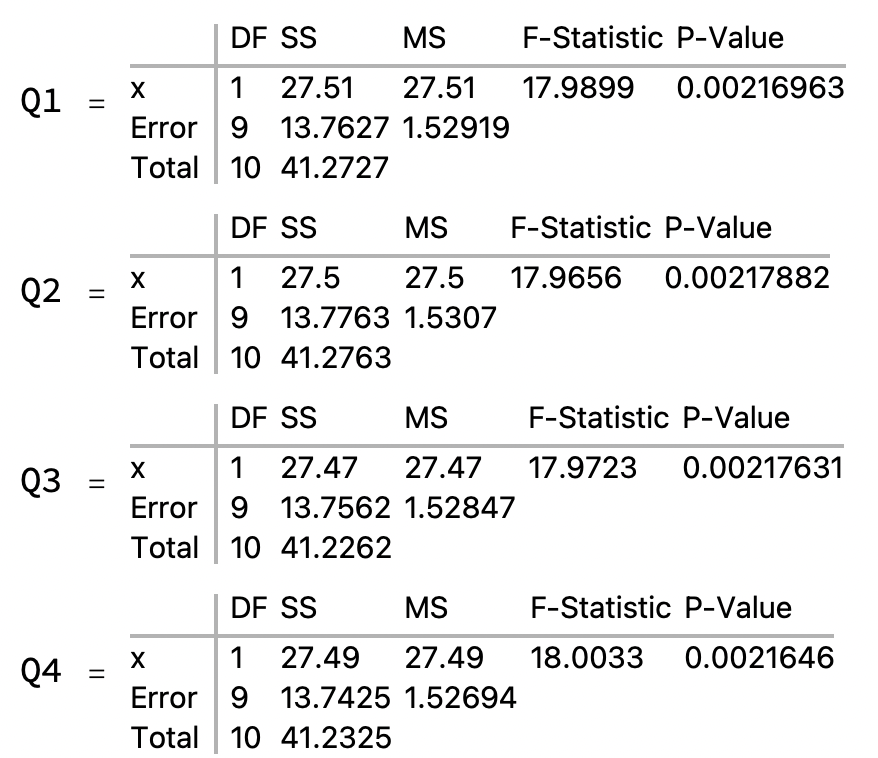
Anscombe’s Quartet
- Anscombe’s Quartet, developed by Francis Anscombe in 1973, consists of four data sets that have almost identical statistics but are very different when graphed.
- wikipedia.org/wiki/Anscombe%27s_quartet
The Graphs


The Stats