• How I became a philosopher
  • I had an irreligious experience

• Nature of Philosophy
  • Subject Matter: Any Fundamental Issue
  • Method: Analysis of Arguments
  • Mindset: Skepticism

• Examples of Arguments
  • President John Oliver
  • Black Swans
  • Editorial on Capital Punishment
  • Declaration of Independence

• Most Important Things about Arguments

• Philosophic Arguments
  • Abortion
    • JJ Thomson’s Famous Violinist Thought Experiment
      • Is there anything wrong with THiS analogical argument?
    • Don Marquis’s Deprivation Theory why Killing is Wrong
  • Is it rational to believe the report of a miracle?
    • Hume’s Of Miracles
  • Consciousness
    • Thought Experiment: Gradually replacing living neurons with synthetic facsimiles
  • Persons
    • Derek Parfit’s Split Brain Thought Experiment
  • Free Will and Determinism
    • Is free will incompatible with the human nervous system?
  • Political Philosophy
    • John Rawls’ Original Position
  • Skepticism
    • Brain-in-a-Vat Thought Experiment
  • What is knowledge?
    • Analysis of Knowledge

• Applied Philosophy
  • Application of philosophic analysis to matters of practical concern, e.g. issues in politics, law, medicine, religion, environment, economics, education, science, and technology.
  • Philosophical analysis is applied to:
    • Arguments
    • Claims
    • Decisions
    • Investigations

• Analysis of:
  • Arguments
    • U.S. Justification for Invading Iraq
    • Mueller’s Argument that Trump Obstructed Justice
    • Alitio’s Argument that there is No Constitutional Right to Abortion
    • Argument that the last twelve verses of Mark were not part of the original text
  • Decisions
    • Decision-Making
      • Framework for Decision-Making
      • Example
      • Two Senses of ‘Bad Decision’
    • Decision to Withdraw from the Iran Nuclear Deal
    • Decision (in 1965) to Americanize the War in Vietnam
    • Decision to Build a Border Wall
  • Investigations
    • Investigation
      • Framework for Investigation
    • Mueller Report
    • Durham Report, when it’s released.
    • Report of Select Committee to Investigate the January 6 Attack on the Capitol, when it’s released.
    • Warren Commission Report on the Assassination of President Kennedy
  • Claims
    • Fact Checkers
      • View Fact-Checking Sites
    • Beyond Fact Checkers
      • Claim that the news media is politically biased
      • Claim that some texts are the revealed word of God

• Other Stuff
  • Paradoxes
    • Surprise Exam
    • Newcomb’s Paradox
  • History of Philosophy
    • The Enlightenment
    • Contemporary Analytic Philosophy

Tools for Evaluating Regressions

Statisticians have developed various kinds of tools for evaluating regressions.

Graphics

• Graphics are essential to evaluating regressions. Indeed, different datasets can have nearly the same statistics but look totally different graphically.
  • View Anscombe’s Quartet
• One of the most useful charts for simple linear regression is a scatter plot of the data with regression line.
  • View Scatter Plot with Regression Line
• But graphs have limitations.  For example, graphing the data and equation for a regression with two IV’s requires three dimensions.
  • View 3D Scatter Plot with Regression Plane
• View Regression Graphics

Correlation

• Variables are correlated to the extent that they vary together, in the same or opposite directions.
• Correlation coefficients are useful
  • between an independent variable and the dependent variable
  • among independent variables
• The Correlation Matrix for multiple regression displays all the correlation coefficients between variables, independent and dependent.
  • View Correlation Matrix
• View Correlation

Prediction

• An hypothesis is supported or disproved by its predictions. A regression equation is an hypothesis. So a natural way of evaluating a regression is to assess its predictions for “out-of-sample” data.
• An interesting metric, the Prediction Sum of Squares (PRESS), evaluates a regression by seeing how well regressions on the sample data, minus one datapoint, predict the missing data item.

Residual Metrics

• A residual is the difference, at a given datapoint, between the values of the observed and predicted dependent variable. There are different ways of combing the residuals into a single statistic.
  • View Residual Metrics

Sum-of-Squares Metrics

• The Least Squares Algorithm is a method finding the equation that, given the observed values of the dependent and independent variables, yields the lowest possible residual sum of squares.
• The residual sum of squares, along with other sums of squares, is thus a natural basis for statistics that evaluate regressions.
• View Principle of Sums of Squares
• View R-Squared
• View Adjusted R-Squared
• View ANOVA for Simple Regression
• View ANOVA for Multiple Regression

Standard Error Metrics

• The standard error of an estimate is how statisticians quantify the idea of average error, i.e. as the standard distribution of the estimate’s sampling distribution.
• Of interest in regression are the standard errors of the regression, the mean of the residuals, the coefficients of the independent variables, and the intercept.
• View Standard Errors of the Regression, the Mean, the Independent Variables, and the Intercept

Likelihood Metrics

• A hypothesis is more likely if it better predicts the data than competing hypotheses, other things being equal. 
• Regression likelihood metrics are based on the idea that the more likely the data given the regression equation, the better the regression.
• View Likelihood Metrics

Linear Regression on IMF

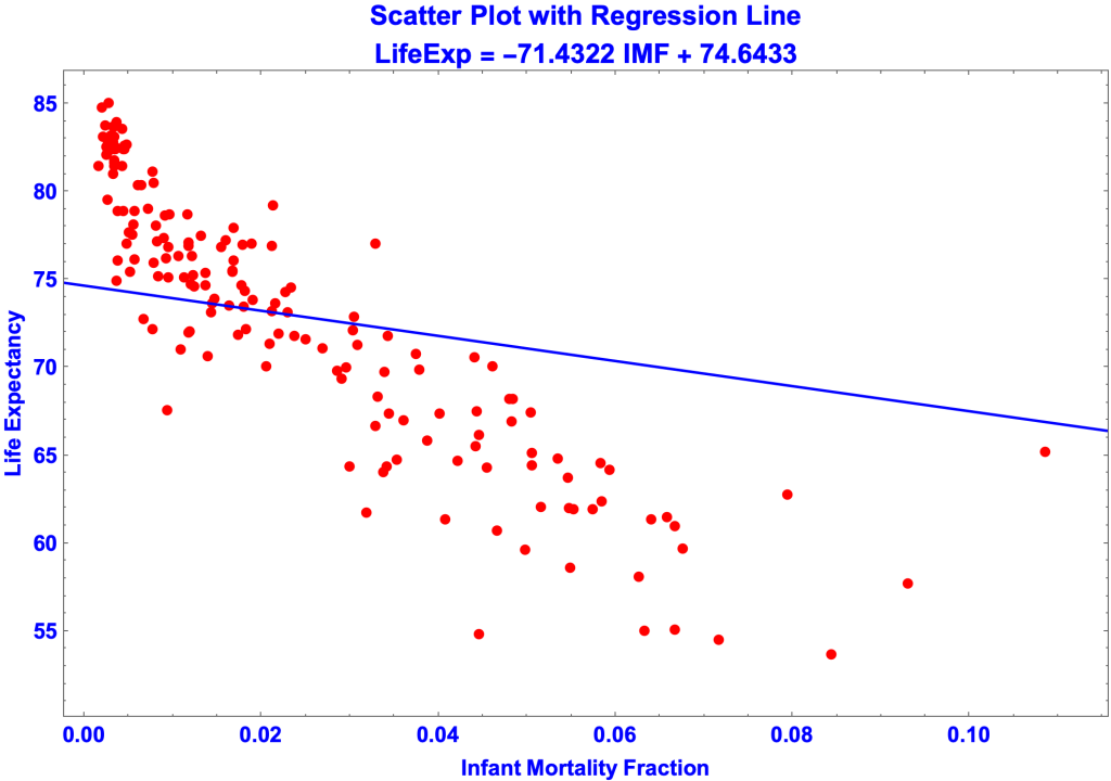
The regression stats are:

• Regression Equation; y = 74.6433 –71.4322 m
• DataPoints = 167
• NbrofIVs = 1
• Sum of Squares Equation: 2369.03 + 7307.92 = 9676.95
  • SSR + SSE = SST, where SSR, SSE, and SST are the sums of squares for
    • predicted y’s
    • residuals
    • observed y’s
• Standard Error of the Regression = 6.6551
  • = √(SSE / (Datapoints – (NbrofIVs + 1)))
• R-Squared = 0.244811
  • = SSR / SST
• Adjusted R-Squared = 0.240234
• AICc = 1111.13

• The regression on IMF is not as good the regression on GDP
  • SER is higher, 6.6551 versus 5.18411.
  • R-Squared is lower, 0.244811 versus 0.541759
  • AICc is higher, 1111.13 versus 1027.7

NonLinear Regression on GDP

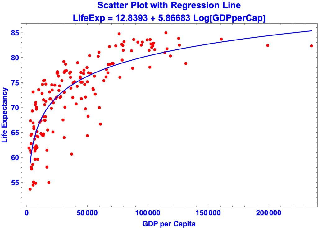
The regression stats:

• Regression Equation; y = 12.8393 + 5.86683 Log[$]
• DataPoints = 167
• NbrofIVs = 1
• Sum of Squares Equation: 6599.56 + 3077.39 = 9676.95
  • SSR + SSE = SST, where SSR, SSE, and SST are the sums of squares for
    • predicted y’s
    • residuals
    • observed y’s
• Standard Error of the Regression = 4.31866
  • = √(SSE / (Datapoints – (NbrofIVs + 1)))
• R-Squared = 0.681988
  • = SSR / SST
• Adjusted R-Squared = 0.68006
• AICc = 966.696

• As you can tell from the scatter plot, this nonlinear regression on GDP is better than its linear counterpart
  • SER is lower, 4.31866 versus 5.18411.
  • R-Squared is higher, 0.681988 versus 0.541759
  • AICc is lower, 966.696 versus 1027.7
• Incidentally, although the regression is nonlinear, R-Squared is valid since SSR and SSE add up to SST. I did my own calculation, since Mathematica calculates nonlinear R-Squareds differently, getting a much higher number, in this case 0.996545.